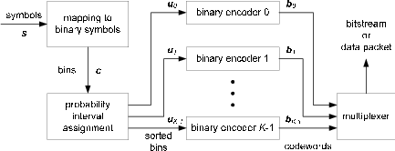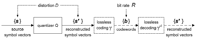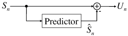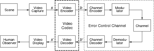
Fig. 1.1 Typical structure of a video transmission system.
This is the html version of the book:
Thomas Wiegand and Heiko Schwarz (2010): "Source Coding: Part I of Fundamentals of Source and Video Coding", Now Publishers, Foundations and Trends® in Signal Processing: Vol. 4: No 1-2, pp 1-222. (pdf version of the book)
1 Introduction
The advances in source coding technology along with the rapid developments and improvements of network infrastructures, storage capacity, and computing power are enabling an increasing number of multimedia applications. In this text, we will describe and analyze fundamental source coding techniques that are found in a variety of multimedia applications, with the emphasis on algorithms that are used in video coding applications. The present first part of the text concentrates on the description of fundamental source coding techniques, while the second part describes their application in modern video coding.
The application areas of digital video today range from multimedia messaging, video telephony, and video conferencing over mobile TV, wireless and wired Internet video streaming, standard- and high-definition TV broadcasting, subscription and pay-per-view services to personal video recorders, digital camcorders, and optical storage media such as the digital versatile disc (DVD) and Blu-Ray disc. Digital video transmission over satellite, cable, and terrestrial channels is typically based on H.222.0/MPEG-2 systems [37], while wired and wireless real-time conversational services often use H.32x [32, 33, 34] or SIP [64], and mobile transmission systems using the Internet and mobile networks are usually based on RTP/IP [68]. In all these application areas, the same basic principles of video compression are employed.
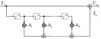
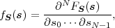
The block structure for a typical video transmission scenario is illustrated in Fig. 1.1. The video capture generates a video signal s that is discrete in space and time. Usually, the video capture consists of a camera that projects the 3-dimensional scene onto an image sensor. Cameras typically generate 25 to 60 frames per second. For the considerations in this text, we assume that the video signal s consists of progressively-scanned pictures. The video encoder maps the video signal s into the bitstream b. The bitstream is transmitted over the error control channel and the received bitstream b′ is processed by the video decoder that reconstructs the decoded video signal s′ and presents it via the video display to the human observer. The visual quality of the decoded video signal s′ as shown on the video display affects the viewing experience of the human observer. This text focuses on the video encoder and decoder part, which is together called a video codec.
The error characteristic of the digital channel can be controlled by the channel encoder, which adds redundancy to the bits at the video encoder output b. The modulator maps the channel encoder output to an analog signal, which is suitable for transmission over a physical channel. The demodulator interprets the received analog signal as a digital signal, which is fed into the channel decoder. The channel decoder processes the digital signal and produces the received bitstream b′, which may be identical to b even in the presence of channel noise. The sequence of the five components, channel encoder, modulator, channel, demodulator, and channel decoder, are lumped into one box, which is called the error control channel. According to Shannon’s basic work [69, 70] that also laid the ground to the subject of this text, by introducing redundancy at the channel encoder and by introducing delay, the amount of transmission errors can be controlled.
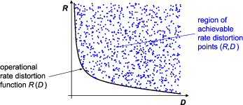
The basic communication problem may be posed as conveying source data with the highest fidelity possible without exceeding an available bit rate, or it may be posed as conveying the source data using the lowest bit rate possible while maintaining a specified reproduction fidelity [69]. In either case, a fundamental trade-off is made between bit rate and signal fidelity. The ability of a source coding system to suitable choose this trade-off is referred to as its coding efficiency or rate distortion performance. Video codecs are thus primarily characterized in terms of:
However, in practical video transmission systems, the following additional issues must be considered:
The practical source coding design problem can be stated as follows: Given a maximum allowed delay and a maximum allowed complexity, achieve an optimal trade-off between bit rate and distortion for the range of network environments envisioned in the scope of the applications.
1.2 Scope and Overview of the Text
This text provides a description of the fundamentals of source and video coding. It is aimed at aiding students and engineers to investigate the subject. When we felt that a result is of fundamental importance to the video codec design problem, we chose to deal with it in greater depth. However, we make no attempt to exhaustive coverage of the subject, since it is too broad and too deep to fit the compact presentation format that is chosen here (and our time limit to write this text). We will also not be able to cover all the possible applications of video coding. Instead our focus is on the source coding fundamentals of video coding. This means that we will leave out a number of areas including implementation aspects of video coding and the whole subject of video transmission and error-robust coding.
The text is divided into two parts. In the first part, the fundamentals of source coding are introduced, while the second part explains their application to modern video coding.
In the present first part, we describe basic source coding techniques that are also found in video codecs. In order to keep the presentation simple, we focus on the description for 1-d discrete-time signals. The extension of source coding techniques to 2-d signals, such as video pictures, will be highlighted in the second part of the text in the context of video coding. Chapter 2 gives a brief overview of the concepts of probability, random variables, and random processes, which build the basis for the descriptions in the following chapters. In Chapter 3, we explain the fundamentals of lossless source coding and present lossless techniques that are found in the video coding area in some detail. The following chapters deal with the topic of lossy compression. Chapter 4 summarizes important results of rate distortion theory, which builds the mathematical basis for analyzing the performance of lossy coding techniques. Chapter 5 treats the important subject of quantization, which can be considered as the basic tool for choosing a trade-off between transmission bit rate and signal fidelity. Due to its importance in video coding, we will mainly concentrate on the description of scalar quantization. But we also briefly introduce vector quantization in order to show the structural limitations of scalar quantization and motivate the later discussed techniques of predictive coding and transform coding. Chapter 6 covers the subject of prediction and predictive coding. These concepts are found in several components of video codecs. Well-known examples are the motion-compensated prediction using previously coded pictures, the intra prediction using already coded samples inside a picture, and the prediction of motion parameters. In Chapter 7, we explain the technique of transform coding, which is used in most video codecs for efficiently representing prediction error signals.
The second part of the text will describe the application of the fundamental source coding techniques to video coding. We will discuss the basic structure and the basic concepts that are used in video coding and highlight their application in modern video coding standards. Additionally, we will consider advanced encoder optimization techniques that are relevant for achieving a high coding efficiency. The effectiveness of various design aspects will be demonstrated based on experimental results.
1.3 The Source Coding Principle
The present first part of the text describes the fundamental concepts of source coding. We explain various known source coding principles and demonstrate their efficiency based on 1-d model sources. For additional information on information theoretical aspects of source coding the reader is referred to the excellent monographs in [11, 22, 4]. For the overall subject of source coding including algorithmic design questions, we recommend the two fundamental texts by Gersho and Gray [16] and Jayant and Noll [44].
The primary task of a source codec is to represent a signal with the minimum number of (binary) symbols without exceeding an “acceptable level of distortion”, which is determined by the application. Two types of source coding techniques are typically named:
Chapter 2 briefly reviews the concepts of probability, random variables, and random processes. Lossless source coding will be described in Chapter 3. The Chapters 5, 6, and 7 give an introduction to the lossy coding techniques that are found in modern video coding applications. In Chapter 4, we provide some important results of rate distortion theory, which will be used for discussing the efficiency of the presented lossy coding techniques.
This is the html version of the book:
Thomas Wiegand and Heiko Schwarz (2010): "Source Coding: Part I of Fundamentals of Source and Video Coding", Now Publishers, Foundations and Trends® in Signal Processing: Vol. 4: No 1-2, pp 1-222.
2 Random Processes
The primary goal of video communication, and signal transmission in general, is the transmission of new information to a receiver. Since the receiver does not know the transmitted signal in advance, the source of information can be modeled as a random process. This permits the description of source coding and communication systems using the mathematical framework of the theory of probability and random processes. If reasonable assumptions are made with respect to the source of information, the performance of source coding algorithms can be characterized based on probabilistic averages. The modeling of information sources as random processes builds the basis for the mathematical theory of source coding and communication.
In this chapter, we give a brief overview of the concepts of probability, random variables, and random processes and introduce models for random processes, which will be used in the following chapters for evaluating the efficiency of the described source coding algorithms. For further information on the theory of probability, random variables, and random processes, the interested reader is referred to [45, 60, 25].
Probability theory is a branch of mathematics, which concerns the description and modeling of random events. The basis for modern probability theory is the axiomatic definition of probability that was introduced by Kolmogorov in [45] using concepts from set theory.
We consider an experiment with an uncertain outcome, which
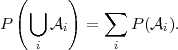
is called a random experiment. The union of all possible outcomes
ζ of the random experiment is referred to as the certain event or
sample space of the random experiment and is denoted by  . A
subset
. A
subset  of the sample space is called an event. To each event a
measure P() is assigned, which is referred to as the probability of the
event . The measure of probability satisfies the following three
axioms:
of the sample space is called an event. To each event a
measure P() is assigned, which is referred to as the probability of the
event . The measure of probability satisfies the following three
axioms:
 | (2.1) |
is equal to 1,
 | (2.2) |
i : i = 0,1, } is a countable set of events
such that i ∩j = ∅ for i≠j, then
} is a countable set of events
such that i ∩j = ∅ for i≠j, then
 | (2.3) |
In addition to the axioms, the notion of the independence of two events and the conditional probability are introduced:
i and j are independent if the probability of their
intersection is the product of their probabilities,
 | (2.4) |
i given another
event j, with P(j) > 0, is denoted by P(i|j) and is defined
as
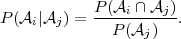 | (2.5) |
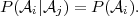
The definitions (2.4) and (2.5) imply that, if two events i and j
are independent and P(j) > 0, the conditional probability of the
event i given the event j is equal to the marginal probability
of i,
 | (2.6) |
A direct consequence of the definition of conditional probability in (2.5) is Bayes’ theorem,
 | (2.7) |
which described the interdependency of the conditional probabilities
P(i|j) and P(j|i) for two events i and j.
A concept that we will use throughout this text are random variables,
which will be denoted with upper-case letters. A random variable S is a
function of the sample space that assigns a real value S(ζ) to each
outcome ζ ∈ of a random experiment.
The cumulative distribution function (cdf) of a random variable S is denoted by FS(s) and specifies the probability of the event {S ≤s},
 | (2.8) |
The cdf is a non-decreasing function with FS(-∞) = 0 and FS(∞) = 1.
The concept of defining a cdf can be extended to sets of two or more
random variables S = {S0, ,SN-1}. The function
 | (2.9) |
is referred to as N-dimensional cdf, joint cdf, or joint distribution. A set S
of random variables is also referred to as a random vector and is also
denoted using the vector notation S = (S0, ,SN-1)T . For the
joint cdf of two random variables X and Y we will use the notation
FXY (x,y) = P(X ≤ x,Y ≤ y). The joint cdf of two random vectors X and
Y will be denoted by FXY (x,y) = P(X ≤ x,Y ≤ y).
,SN-1)T . For the
joint cdf of two random variables X and Y we will use the notation
FXY (x,y) = P(X ≤ x,Y ≤ y). The joint cdf of two random vectors X and
Y will be denoted by FXY (x,y) = P(X ≤ x,Y ≤ y).
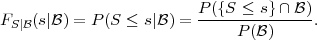
The conditional cdf or conditional distribution of a random variable S
given an event  , with P() > 0, is defined as the conditional probability
of the event {S ≤ s} given the event ,
, with P() > 0, is defined as the conditional probability
of the event {S ≤ s} given the event ,
 | (2.10) |
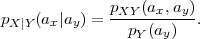
The conditional distribution of a random variable X given another random variable Y is denoted by FX|Y (x|y) and defined as
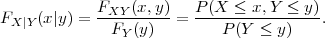 | (2.11) |
Similarly, the conditional cdf of a random vector X given another random vector Y is given by FX|Y (x|y) = FXY (x,y)∕FY (y).
2.2.1 Continuous Random Variables
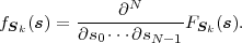
A random variable S is called a continuous random variable, if its cdf FS(s) is a continuous function. The probability P(S = s) is equal to zero for all values of s. An important function of continuous random variables is the probability density function (pdf), which is defined as the derivative of the cdf,
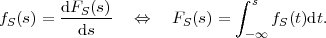 | (2.12) |
Since the cdf FS(s) is a monotonically non-decreasing function, the pdf fS(s) is greater than or equal to zero for all values of s. Important examples for pdf’s, which we will use later in this text, are given below.
Uniform pdf:
 | (2.13) |
Laplacian pdf:
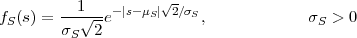 | (2.14) |
Gaussian pdf:
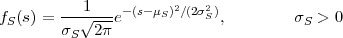 | (2.15) |
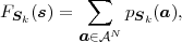
The concept of defining a probability density function is also extended to
random vectors S = (S0, ,SN-1)T . The multivariate derivative of the
joint cdf FS(s),
,SN-1)T . The multivariate derivative of the
joint cdf FS(s),
 | (2.16) |
is referred to as the N-dimensional pdf, joint pdf, or joint density. For two random variables X and Y , we will use the notation fXY (x,y) for denoting the joint pdf of X and Y . The joint density of two random vectors X and Y will be denoted by fXY (x,y).
The conditional pdf or conditional density fS| (s|) of a random
variable S given an event , with P() > 0, is defined as the derivative of
the conditional distribution FS|(s|), fS|(s|) = dFS|(s|)∕ds. The
conditional density of a random variable X given another random
variable Y is denoted by fX|Y (x|y) and defined as
(s|) of a random
variable S given an event , with P() > 0, is defined as the derivative of
the conditional distribution FS|(s|), fS|(s|) = dFS|(s|)∕ds. The
conditional density of a random variable X given another random
variable Y is denoted by fX|Y (x|y) and defined as
 | (2.17) |
Similarly, the conditional pdf of a random vector X given another random vector Y is given by fX|Y (x|y) = fXY (x,y)∕fY (y).
2.2.2 Discrete Random Variables
A random variable S is said to be a discrete random variable if its
cdf FS(s) represents a staircase function. A discrete random variable S can
only take values of a countable set = {a0,a1,…}, which is called the
alphabet of the random variable. For a discrete random variable S with an
alphabet , the function
 | (2.18) |
which gives the probabilities that S is equal to a particular alphabet letter, is referred to as probability mass function (pmf). The cdf FS(s) of a discrete random variable S is given by the sum of the probability masses p(a) with a ≤ s,
 | (2.19) |
With the Dirac delta function δ it is also possible to use a pdf fS for describing the statistical properties of a discrete random variables S with a pmf pS(a),
 | (2.20) |
Examples for pmf’s that will be used in this text are listed below. The pmf’s are specified in terms of parameters p and M, where p is a real number in the open interval (0,1) and M is an integer greater than 1. The binary and uniform pmf are specified for discrete random variables with a finite alphabet, while the geometric pmf is specified for random variables with a countably infinite alphabet.
Binary pmf:
 | (2.21) |
Uniform pmf:
 | (2.22) |
Geometric pmf:
 | (2.23) |
The pmf for a random vector S = (S0, ,SN-1)T is defined by
 | (2.24) |
and is also referred to as N-dimensional pmf or joint pmf. The joint pmf for two random variables X and Y or two random vectors X and Y will be denoted by pXY (ax,ay) or pXY (ax,ay), respectively.
The conditional pmf pS|(a|) of a random variable S given an event ,
with P() > 0, specifies the conditional probabilities of the events {S = a}
given the event B, pS|(a|) = P(S = a|). The conditional pmf of a
random variable X given another random variable Y is denoted by
pX|Y (ax|ay) and defined as
 | (2.25) |
Similarly, the conditional pmf of a random vector X given another random vector Y is given by pX|Y (ax|ay) = pXY (ax,ay)∕pY (ay).
Statistical properties of random variables are often expressed using probabilistic averages, which are referred to as expectation values or expected values. The expectation value of an arbitrary function g(S) of a continuous random variable S is defined by the integral
 | (2.26) |
For discrete random variables S, it is defined as the sum
 | (2.27) |
Two important expectation values are the mean μS and the variance σS2 of a random variable S, which are given by
 | (2.28) |
For the following discussion of expectation values, we consider continuous random variables. For discrete random variables, the integrals have to be replaced by sums and the pdf’s have to be replaced by pmf’s.
The expectation value of a function g(S) of a set N random variables
S = {S0, ,SN-1} is given by
 | (2.29) |
The conditional expectation value of a function g(S) of a random
variable S given an event , with P() > 0, is defined by
 | (2.30) |
The conditional expectation value of a function g(X) of random variable X given a particular value y for another random variable Y is specified by
 | (2.31) |
and represents a deterministic function of the value y. If the value y is
replaced by the random variable Y , the expression E specifies a
new random variable that is a function of the random variable Y . The
expectation value E
specifies a
new random variable that is a function of the random variable Y . The
expectation value E of a random variable Z = E
 can be
computed using the iterative expectation rule,
can be
computed using the iterative expectation rule,
We now consider a series of random experiments that are performed at time instants tn, with n being an integer greater than or equal to 0. The outcome of each random experiment at a particular time instant tn is characterized by a random variable Sn = S(tn). The series of random variables S = {Sn} is called a discrete-time1 random process. The statistical properties of a discrete-time random process S can be characterized by the N-th order joint cdf
 | (2.33) |
Random processes S that represent a series of continuous random variables Sn are called continuous random processes and random processes for which the random variables Sn are of discrete type are referred to as discrete random processes. For continuous random processes, the statistical properties can also be described by the N-th order joint pdf, which is given by the multivariate derivative
 | (2.34) |
For discrete random processes, the N-th order joint cdf FSk(s) can also be specified using the N-th order joint pmf,
 | (2.35) |
where N represent the product space of the alphabets n for the random
variables Sn with n = k, ,k + N - 1 and
 | (2.36) |
represents the N-th order joint pmf.
The statistical properties of random processes S = {Sn} are often characterized by an N-th order autocovariance matrix CN(tk) or an N-th order autocorrelation matrix RN(tk). The N-th order autocovariance matrix is defined by
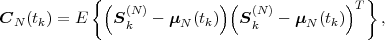 | (2.37) |
where Sk(N) represents the vector (Sk, ,Sk+N-1)T of N successive
random variables and μN(tk) = E
,Sk+N-1)T of N successive
random variables and μN(tk) = E Sk(N)
Sk(N) is the N-th order mean. The
N-th order autocorrelation matrix is defined by
is the N-th order mean. The
N-th order autocorrelation matrix is defined by
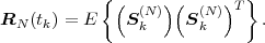 | (2.38) |
A random process is called stationary if its statistical properties are invariant to a shift in time. For stationary random processes, the N-th order joint cdf FSk(s), pdf fSk(s), and pmf pSk(a) are independent of the first time instant tk and are denoted by FS(s), fS(s), and pS(a), respectively. For the random variables Sn of stationary processes we will often omit the index n and use the notation S.
For stationary random processes, the N-th order mean, the N-th order
autocovariance matrix, and the N-th order autocorrelation matrix are
independent of the time instant tk and are denoted by μN, CN, and RN,
respectively. The N-th order mean μN is a vector with all N elements being
equal to the mean μS of the random variables S. The N-th order
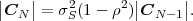
autocovariance matrix CN = E (S(N) -μN)(S(N) -μN)T
  is a
symmetric Toeplitz matrix,
is a
symmetric Toeplitz matrix,
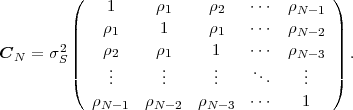 | (2.39) |
A Toepliz matrix is a matrix with constant values along all descending
diagonals from left to right. For information on the theory and application
of Toeplitz matrices the reader is referred to the standard reference [29]
and the tutorial [23]. The (k,l)-th element of the autocovariance matrix
CN is given by the autocovariance function ϕk,l = E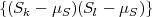 .
For stationary processes, the autocovariance function depends only on the
absolute values |k - l| and can be written as ϕk,l = ϕ|k-l| = σS2ρ|k-l|. The
N-th order autocorrelation matrix RN is also is symmetric Toeplitz matrix.
The (k,l)-th element of RN is given by rk,l = ϕk,l + μS2.
.
For stationary processes, the autocovariance function depends only on the
absolute values |k - l| and can be written as ϕk,l = ϕ|k-l| = σS2ρ|k-l|. The
N-th order autocorrelation matrix RN is also is symmetric Toeplitz matrix.
The (k,l)-th element of RN is given by rk,l = ϕk,l + μS2.
A random process S = {Sn} for which the random variables Sn are
independent is referred to as memoryless random process. If a memoryless
random process is additionally stationary it is also said to be independent
and identical distributed (iid), since the random variables Sn are
independent and their cdf’s FSn(s) = P(Sn ≤ s) do not depend on the time
instant tn. The N-th order cdf FS(s), pdf fS(s), and pmf pS(a) for iid
processes, with s = (s0, ,sN-1)T and a = (a0,
 ,aN-1)T , are given by
the products
,aN-1)T , are given by
the products
 | (2.40) |
where FS(s), fS(s), and pS(a) are the marginal cdf, pdf, and pmf, respectively, for the random variables Sn.
A Markov process is characterized by the property that future outcomes do not depend on past outcomes, but only on the present outcome,
 | (2.41) |
This property can also be expressed in terms of the pdf,
 | (2.42) |
for continuous random processes, or in terms of the pmf,
 | (2.43) |
for discrete random processes,
Given a continuous zero-mean iid process Z = {Zn}, a stationary continuous Markov process S = {Sn} with mean μS can be constructed by the recursive rule
 | (2.44) |
where ρ, with |ρ| < 1, represents the correlation coefficient between successive random variables Sn-1 and Sn. Since the random variables Zn are independent, a random variable Sn only depends on the preceding random variable Sn-1. The variance σS2 of the stationary Markov process S is given by
 | (2.45) |
where σZ2 = E denotes the variance of the zero-mean iid process Z.
The autocovariance function of the process S is given by
denotes the variance of the zero-mean iid process Z.
The autocovariance function of the process S is given by
 | (2.46) |
Each element ϕk,l of the N-th order autocorrelation matrix CN represents a non-negative integer power of the correlation coefficient ρ.
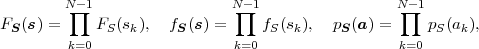
In following chapters, we will often obtain expressions that depend on the determinant |CN| of the N-th order autocovariance matrix CN. For stationary continuous Markov processes given by (2.44), the determinant |CN| can be expressed by a simple relationship. Using Laplace’s formula, we can expand the determinant of the N-th order autocovariance matrix along the first column,
 | (2.47) |
where CN(k,l) represents the matrix that is obtained by removing the k-th row and l-th column from CN. The first row of each matrix CN(k,l), with k > 1, is equal to the second row of the same matrix multiplied by the correlation coefficient ρ. Hence, the first two rows of these matrices are linearly dependent and the determinants |CN(k,l)|, with k > 1, are equal to 0. Thus, we obtain
 | (2.48) |
The matrix CN(0,0) represents the autocovariance matrix CN-1 of the order (N - 1). The matrix CN(1,0) is equal to CN-1 except that the first row is multiplied by the correlation coefficient ρ. Hence, the determinant |CN(1,0)| is equal to ρ|CN-1|, which yields the recursive rule
 | (2.49) |
By using the expression |C1| = σS2 for the determinant of the 1-st order autocovariance matrix, we obtain the relationship
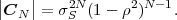 | (2.50) |
A continuous random process S = {Sn} is said to be a Gaussian process if all finite collections of random variables Sn represent Gaussian random vectors. The N-th order pdf of a stationary Gaussian process S with mean μS and variance σS2 is given by
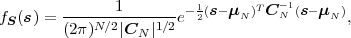 | (2.51) |
where s is a vector of N consecutive samples, μN is the N-th order mean (a vector with all N elements being equal to the mean μS), and CN is an N-th order nonsingular autocovariance matrix given by (2.39).
A continuous random process is called a Gauss-Markov process if it satisfies the requirements for both Gaussian processes and Markov processes. The statistical properties of a stationary Gauss-Markov are completely specified by its mean μS, its variance σS2, and its correlation coefficient ρ. The stationary continuous process in (2.44) is a stationary Gauss-Markov process if the random variables Zn of the zero-mean iid process Z have a Gaussian pdf fZ(s).
The N-th order pdf of a stationary Gauss-Markov process S with the mean μS, the variance σS2, and the correlation coefficient ρ is given by (2.51), where the elements ϕk,l of the N-th order autocovariance matrix CN depend on the variance σS2 and the correlation coefficient ρ and are given by (2.46). The determinant |CN| of the N-th order autocovariance matrix of a stationary Gauss-Markov process can be written according to (2.50).
2.4 Summary of Random Processes
In this chapter, we gave a brief review of the concepts of random variables and random processes. A random variable is a function of the sample space of a random experiment. It assigns a real value to each possible outcome of the random experiment. The statistical properties of random variables can be characterized by cumulative distribution functions (cdf’s), probability density functions (pdf’s), probability mass functions (pmf’s), or expectation values.
Finite collections of random variables are called random vectors. A countably infinite sequence of random variables is referred to as (discrete-time) random process. Random processes for which the statistical properties are invariant to a shift in time are called stationary processes. If the random variables of a process are independent, the process is said to be memoryless. Random processes that are stationary and memoryless are also referred to as independent and identically distributed (iid) processes. Important models for random processes, which will also be used in this text, are Markov processes, Gaussian processes, and Gauss-Markov processes.
Beside reviewing the basic concepts of random variables and random processes, we also introduced the notations that will be used throughout the text. For simplifying formulas in the following chapters, we will often omit the subscripts that characterize the random variable(s) or random vector(s) in the notations of cdf’s, pdf’s, and pmf’s.
This is the html version of the book:
Thomas Wiegand and Heiko Schwarz (2010): "Source Coding: Part I of Fundamentals of Source and Video Coding", Now Publishers, Foundations and Trends® in Signal Processing: Vol. 4: No 1-2, pp 1-222.
3 Lossless Source Coding
Lossless source coding describes a reversible mapping of sequences of discrete source symbols into sequences of codewords. In contrast to lossy coding techniques, the original sequence of source symbols can be exactly reconstructed from the sequence of codewords. Lossless coding is also referred to as noiseless coding or entropy coding. If the original signal contains statistical properties or dependencies that can be exploited for data compression, lossless coding techniques can provide a reduction in transmission rate. Basically all source codecs, and in particular all video codecs, include a lossless coding part by which the coding symbols are efficiently represented inside a bitstream.
In this chapter, we give an introduction to lossless source coding. We analyze the requirements for unique decodability, introduce a fundamental bound for the minimum average codeword length per source symbol that can be achieved with lossless coding techniques, and discuss various lossless source codes with respect to their efficiency, applicability, and complexity. For further information on lossless coding techniques, the reader is referred to the overview of lossless compression techniques in [67].
3.1 Classification of Lossless Source Codes
In this text, we restrict our considerations to the practically important case
of binary codewords. A codeword is a sequence of binary symbols (bits)
of the alphabet = {0,1}. Let S = {Sn} be a stochastic process
that generates sequences of discrete source symbols. The source
symbols sn are realizations of the random variables Sn. By the process of
lossless coding, a message s(L) = {s0, ,sL-1} consisting of L source
symbols is converted into a sequence b(K) = {b0,
,sL-1} consisting of L source
symbols is converted into a sequence b(K) = {b0, ,bK-1} of K
bits.
,bK-1} of K
bits.
In practical coding algorithms, a message s(L) is often split into blocks
s(N) = {sn, ,sn+N-1} of N symbols, with 1 ≤ N ≤ L, and a codeword
b(ℓ)(s(N)) = {b0,
,sn+N-1} of N symbols, with 1 ≤ N ≤ L, and a codeword
b(ℓ)(s(N)) = {b0, ,bℓ-1} of ℓ bits is assigned to each of these blocks s(N).
The length ℓ of a codeword bℓ(s(N)) can depend on the symbol block s(N).
The codeword sequence b(K) that represents the message s(L) is
obtained by concatenating the codewords bℓ(s(N)) for the symbol
blocks s(N). A lossless source code can be described by the encoder
mapping
,bℓ-1} of ℓ bits is assigned to each of these blocks s(N).
The length ℓ of a codeword bℓ(s(N)) can depend on the symbol block s(N).
The codeword sequence b(K) that represents the message s(L) is
obtained by concatenating the codewords bℓ(s(N)) for the symbol
blocks s(N). A lossless source code can be described by the encoder
mapping
 | (3.1) |
which specifies a mapping from the set of finite length symbol blocks to the set of finite length binary codewords. The decoder mapping
 | (3.2) |
is the inverse of the encoder mapping γ.
Depending on whether the number N of symbols in the blocks s(N) and the number ℓ of bits for the associated codewords are fixed or variable, the following categories can be distinguished:
3.2 Variable-Length Coding for Scalars
In this section, we consider lossless source codes that assign a separate
codeword to each symbol sn of a message s(L). It is supposed that the
symbols of the message s(L) are generated by a stationary discrete random
process S = {Sn}. The random variables Sn = S are characterized by a
finite11 The fundamental concepts and results shown in this section are also valid for countably infinite
symbol alphabets (M →∞).
symbol alphabet = {a0, ,aM-1} and a marginal pmf p(a) = P(S = a).
The lossless source code associates each letter ai of the alphabet with a
binary codeword bi = {b0i,
,aM-1} and a marginal pmf p(a) = P(S = a).
The lossless source code associates each letter ai of the alphabet with a
binary codeword bi = {b0i, ,bℓ(ai)-1i} of a length ℓ(ai) ≥ 1. The
goal of the lossless code design is to minimize the average codeword
length
,bℓ(ai)-1i} of a length ℓ(ai) ≥ 1. The
goal of the lossless code design is to minimize the average codeword
length
 | (3.3) |
while ensuring that each message s(L) is uniquely decodable given their coded representation b(K).
A code is said to be uniquely decodable if and only if each valid coded representation b(K) of a finite number K of bits can be produced by only one possible sequence of source symbols s(L).
A necessary condition for unique decodability is that each letter ai of
the symbol alphabet is associated with a different codeword. Codes
with this property are called non-singular codes and ensure that a
single source symbol is unambiguously represented. But if messages
with more than one symbol are transmitted, non-singularity is not
sufficient to guarantee unique decodability, as will be illustrated in the
following.
Table 3.1 shows five example codes for a source with a four letter alphabet and a given marginal pmf. Code A has the smallest average codeword length, but since the symbols a2 and a3 cannot be distinguished2. Code A is a singular code and is not uniquely decodable. Although code B is a non-singular code, it is not uniquely decodable either, since the concatenation of the letters a1 and a0 produces the same bit sequence as the letter a2. The remaining three codes are uniquely decodable, but differ in other properties. While code D has an average codeword length of 2.125 bit per symbol, the codes C and E have an average codeword length of only 1.75 bit per symbol, which is, as we will show later, the minimum achievable average codeword length for the given source. Beside being uniquely decodable, the codes D and E are also instantaneously decodable, i.e., each alphabet letter can be decoded right after the bits of its codeword are received. The code C does not have this property. If a decoder for the code C receives a bit equal to 0, it has to wait for the next bit equal to 0 before a symbol can be decoded. Theoretically, the decoder might need to wait until the end of the message. The value of the next symbol depends on how many bits equal to 1 are received between the zero bits.
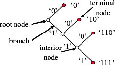
Binary codes can be represented using binary trees as illustrated in Fig. 3.1. A binary tree is a data structure that consists of nodes, with each node having zero, one, or two descendant nodes. A node and its descendants nodes are connected by branches. A binary tree starts with a root node, which is the only node that is not a descendant of any other node. Nodes that are not the root node but have descendants are referred to as interior nodes, whereas nodes that do not have descendants are called terminal nodes or leaf nodes.
In a binary code tree, all branches are labeled with ‘0’ or ‘1’. If two
branches depart from the same node, they have different labels. Each node
of the tree represents a codeword, which is given by the concatenation of
the branch labels from the root node to the considered node. A
code for a given alphabet can be constructed by associating all
terminal nodes and zero or more interior nodes of a binary code
tree with one or more alphabet letters. If each alphabet letter is
associated with a distinct node, the resulting code is non-singular. In the
example of Fig. 3.1, the nodes that represent alphabet letters are
filled.
A code is said to be a prefix code if no codeword for an alphabet letter represents the codeword or a prefix of the codeword for any other alphabet letter. If a prefix code is represented by a binary code tree, this implies that each alphabet letter is assigned to a distinct terminal node, but not to any interior node. It is obvious that every prefix code is uniquely decodable. Furthermore, we will prove later that for every uniquely decodable code there exists a prefix code with exactly the same codeword lengths. Examples for prefix codes are the codes D and E in Table 3.1.
Based on the binary code tree representation the parsing rule for prefix codes can be specified as follows:
The parsing rule reveals that prefix codes are not only uniquely decodable, but also instantaneously decodable. As soon as all bits of a codeword are received, the transmitted symbol is immediately known. Due to this property, it is also possible to switch between different independently designed prefix codes inside a bitstream (i.e., because symbols with different alphabets are interleaved according to a given bitstream syntax) without impacting the unique decodability.
A necessary condition for uniquely decodable codes is given by the Kraft inequality,
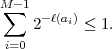 | (3.4) |
For proving this inequality, we consider the term
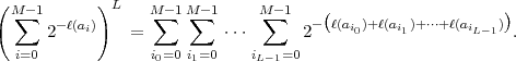 | (3.5) |
The term ℓL = ℓ(ai0) + ℓ(ai1) +  + ℓ(aiL-1) represents the combined
codeword length for coding L symbols. Let A(ℓL) denote the number
of distinct symbol sequences that produce a bit sequence with the
same length ℓL. A(ℓL) is equal to the number of terms 2-ℓL that are
contained in the sum of the right side of (3.5). For a uniquely decodable
code, A(ℓL) must be less than or equal to 2ℓL, since there are only
2ℓL distinct bit sequences of length ℓL. If the maximum length of a
codeword is ℓmax, the combined codeword length ℓL lies inside the
interval [L,L ⋅ ℓmax]. Hence, a uniquely decodable code must fulfill the
inequality
+ ℓ(aiL-1) represents the combined
codeword length for coding L symbols. Let A(ℓL) denote the number
of distinct symbol sequences that produce a bit sequence with the
same length ℓL. A(ℓL) is equal to the number of terms 2-ℓL that are
contained in the sum of the right side of (3.5). For a uniquely decodable
code, A(ℓL) must be less than or equal to 2ℓL, since there are only
2ℓL distinct bit sequences of length ℓL. If the maximum length of a
codeword is ℓmax, the combined codeword length ℓL lies inside the
interval [L,L ⋅ ℓmax]. Hence, a uniquely decodable code must fulfill the
inequality
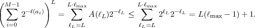 | (3.6) |
The left side of this inequality grows exponentially with L, while the right side grows only linearly with L. If the Kraft inequality (3.4) is not fulfilled, we can always find a value of L for which the condition (3.6) is violated. And since the constraint (3.6) must be obeyed for all values of L ≥ 1, this proves that the Kraft inequality specifies a necessary condition for uniquely decodable codes.
The Kraft inequality does not only provide a necessary condition for
uniquely decodable codes, it is also always possible to construct a uniquely
decodable code for any given set of codeword lengths {ℓ0,ℓ1, ,ℓM-1} that
satisfies the Kraft inequality. We prove this statement for prefix codes,
which represent a subset of uniquely decodable codes. Without loss of
generality, we assume that the given codeword lengths are ordered as
ℓ0 ≤ ℓ1 ≤
,ℓM-1} that
satisfies the Kraft inequality. We prove this statement for prefix codes,
which represent a subset of uniquely decodable codes. Without loss of
generality, we assume that the given codeword lengths are ordered as
ℓ0 ≤ ℓ1 ≤ ≤ ℓM-1. Starting with an infinite binary code tree, we
chose an arbitrary node of depth ℓ0 (i.e., a node that represents a
codeword of length ℓ0) for the first codeword and prune the code tree at
this node. For the next codeword length ℓ1, one of the remaining
nodes with depth ℓ1 is selected. A continuation of this procedure
yields a prefix code for the given set of codeword lengths, unless we
cannot select a node for a codeword length ℓi because all nodes of
depth ℓi have already been removed in previous steps. It should be
noted that the selection of a codeword of length ℓk removes 2ℓi-ℓk
codewords with a length of ℓi ≥ ℓk. Consequently, for the assignment of
a codeword length ℓi, the number of available codewords is given
by
≤ ℓM-1. Starting with an infinite binary code tree, we
chose an arbitrary node of depth ℓ0 (i.e., a node that represents a
codeword of length ℓ0) for the first codeword and prune the code tree at
this node. For the next codeword length ℓ1, one of the remaining
nodes with depth ℓ1 is selected. A continuation of this procedure
yields a prefix code for the given set of codeword lengths, unless we
cannot select a node for a codeword length ℓi because all nodes of
depth ℓi have already been removed in previous steps. It should be
noted that the selection of a codeword of length ℓk removes 2ℓi-ℓk
codewords with a length of ℓi ≥ ℓk. Consequently, for the assignment of
a codeword length ℓi, the number of available codewords is given
by
 | (3.7) |
If the Kraft inequality (3.4) is fulfilled, we obtain
 | (3.8) |
Hence, it is always possible to construct a prefix code, and thus a uniquely decodable code, for a given set of codeword lengths that satisfies the Kraft inequality.
The proof shows another important property of prefix codes. Since all uniquely decodable codes fulfill the Kraft inequality and it is always possible to construct a prefix code for any set of codeword lengths that satisfies the Kraft inequality, there do not exist uniquely decodable codes that have a smaller average codeword length than the best prefix code. Due to this property and since prefix codes additionally provide instantaneous decodability and are easy to construct, all variable length codes that are used in practice are prefix codes.
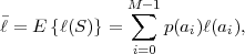
Based on the Kraft inequality, we now derive a lower bound for the average codeword length of uniquely decodable codes. The expression (3.3) for the average codeword length can be rewritten as
 | (3.9) |
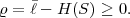
With the definition q(ai) = 2-ℓ(ai)∕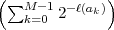 , we obtain
 | (3.10) |
Since the Kraft inequality is fulfilled for all uniquely decodable codes, the first term on the right side of (3.10) is greater than or equal to 0. The second term is also greater than or equal to 0 as can be shown using the inequality lnx ≤ x - 1 (with equality if and only if x = 1),
The inequality (3.11) is also referred to as divergence inequality for probability mass functions. The average codeword length for uniquely decodable codes is bounded by
 | (3.12) |
with
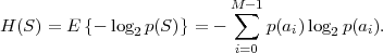 | (3.13) |
The lower bound H(S) is called the entropy of the random variable S and does only depend on the associated pmf p. Often the entropy of a random variable with a pmf p is also denoted as H(p). The redundancy of a code is given by the difference
 | (3.14) |
The entropy H(S) can also be considered as a measure for the uncertainty3 that is associated with the random variable S.
The inequality (3.12) is an equality if and only if the first and second
term on the right side of (3.10) are equal to 0. This is only the case
if the Kraft inequality is fulfilled with equality and q(ai) = p(ai),
∀ai ∈. The resulting conditions ℓ(ai) = -log 2p(ai), ∀ai ∈, can only
hold if all alphabet letters have probabilities that are integer powers
of 1∕2.
For deriving an upper bound for the minimum average codeword length
we choose ℓ(ai) = ⌈-log 2p(ai)⌉, ∀ai ∈, where ⌈x⌉ represents the smallest
integer greater than or equal to x. Since these codeword lengths satisfy the
Kraft inequality, as can be shown using ⌈x⌉≥ x,
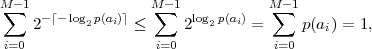 | (3.15) |
we can always construct a uniquely decodable code. For the average codeword length of such a code, we obtain, using ⌈x⌉ < x + 1,
 | (3.16) |
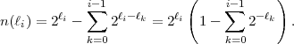
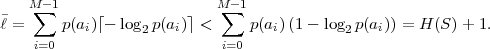
The minimum average codeword length min that can be achieved with uniquely decodable codes that assign a separate codeword to each letter of an alphabet always satisfies the inequality
 | (3.17) |
The upper limit is approached for a source with a two-letter alphabet and a pmf {p,1 - p} if the letter probability p approaches 0 or 1 [15].
For deriving an upper bound for the minimum average codeword
length we chose ℓ(ai) = ⌈-log 2p(ai)⌉, ∀ai ∈. The resulting code
has a redundancy ϱ = - H(Sn) that is always less than 1 bit per
symbol, but it does not necessarily achieve the minimum average
codeword length. For developing an optimal uniquely decodable code,
i.e., a code that achieves the minimum average codeword length,
it is sufficient to consider the class of prefix codes, since for every
uniquely decodable code there exists a prefix code with the exactly
same codeword length. An optimal prefix code has the following
properties:
with p(ai) > p(aj), the
associated codeword lengths satisfy ℓ(ai) ≤ℓ(aj).
These conditions can be proved as follows. If the first condition is not fulfilled, an exchange of the codewords for the symbols ai and aj would decrease the average codeword length while preserving the prefix property. And if the second condition is not satisfied, i.e., if for a particular codeword with the maximum codeword length there does not exist a codeword that has the same length and differs only in the final bit, the removal of the last bit of the particular codeword would preserve the prefix property and decrease the average codeword length.
Both conditions for optimal prefix codes are obeyed if two codewords
with the maximum length that differ only in the final bit are assigned
to the two letters ai and aj with the smallest probabilities. In the
corresponding binary code tree, a parent node for the two leaf nodes that
represent these two letters is created. The two letters ai and aj can then be
treated as a new letter with a probability of p(ai) + p(aj) and the procedure
of creating a parent node for the nodes that represent the two letters with
the smallest probabilities can be repeated for the new alphabet. The
resulting iterative algorithm was developed and proved to be optimal by
Huffman in [30]. Based on the construction of a binary code tree, the
Huffman algorithm for a given alphabet with a marginal pmf p can be
summarized as follows:
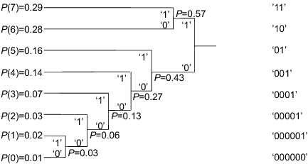
Adetailed example for the application of the Huffman algorithm is given in Fig. 3.2. Optimal prefix codes are often generally referred to as Huffman codes. It should be noted that there exist multiple optimal prefix codes for a given marginal pmf. A tighter bound than in (3.17) on the redundancy of Huffman codes is provided in [15].
3.2.4 Conditional Huffman Codes
Until now, we considered the design of variable length codes for the marginal pmf of stationary random processes. However, for random processes {Sn} with memory, it can be beneficial to design variable length codes for conditional pmfs and switch between multiple codeword tables depending on already coded symbols.
| a | a0 | a1 | a2 | entropy
|
| p(a|a0) | 0.90 | 0.05 | 0.05 | H(Sn|a0) = 0.5690 |
| p(a|a1) | 0.15 | 0.80 | 0.05 | H(Sn|a1) = 0.8842 |
| p(a|a2) | 0.25 | 0.15 | 0.60 | H(Sn|a2) = 1.3527 |
| p(a) | 0.64 | 0.24 | 0.1 | H(S) = 1.2575 |
As an example, we consider a stationary discrete Markov process with a
three symbol alphabet = {a0,a1,a2}. The statistical properties of
this process are completely characterized by three conditional pmfs
p(a|ak) = P(Sn = a|Sn-1 = ak) with k = 0,1,2, which are given in
Table 3.2. An optimal prefix code for a given conditional pmf can be
designed in exactly the same way as for a marginal pmf. A corresponding
Huffman code design for the example Markov source is shown in Table 3.3.
For comparison, Table 3.3 lists also a Huffman code for the marginal
pmf. The codeword table that is chosen for coding a symbol sn
depends on the value of the preceding symbol sn-1. It is important to
note that an independent code design for the conditional pmfs is
only possible for instantaneously decodable codes, i.e., for prefix
codes.
|
ai | Huffman codes for conditional pmfs |
|
||||
| Sn-1 = a0 | Sn-1 = a2 | Sn-1 = a2 | ||||
| a 0 | 1 | 00 | 00 | 1 | ||
| a 1 | 00 | 1 | 01 | 00 | ||
| a 2 | 01 | 01 | 1 | 01 | ||
| 1.1 | 1.2 | 1.4 | 1.3556 | |||
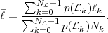
The average codeword length k = (Sn-1 = ak) of an optimal prefix
code for each of the conditional pmfs is guaranteed to lie in the half-open
interval  , where
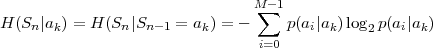 | (3.18) |
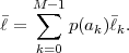
denotes the conditional entropy of the random variable Sn given the event {Sn-1 = ak}. The resulting average codeword length for the conditional code is
 | (3.19) |
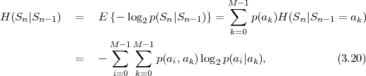
The resulting lower bound for the average codeword length is referred to as the conditional entropy H(Sn|Sn-1) of the random variable Sn assuming the random variable Sn-1 and is given by
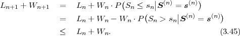
where p(ai,ak) = P(Sn = ai,Sn-1 = ak) denotes the joint pmf of the random variables Sn and Sn-1. The conditional entropy H(Sn|Sn-1) specifies a measure for the uncertainty about Sn given the value of Sn-1. The minimum average codeword length min that is achievable with the conditional code design is bounded by
 | (3.21) |
As can be easily shown from the divergence inequality (3.11),
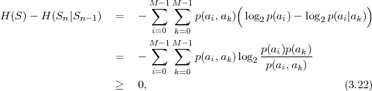 , i.e., if the stationary process S is an iid process.
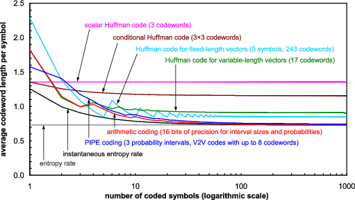
For our example, the average codeword length of the conditional code design is 1.1578 bit per symbol, which is about 14.6% smaller than the average codeword length of the Huffman code for the marginal pmf.
For sources with memory that do not satisfy the Markov property, it can be possible to further decrease the average codeword length if more than one preceding symbol is used in the condition. However, the number of codeword tables increases exponentially with the number of considered symbols. To reduce the number of tables, the number of outcomes for the condition can be partitioned into a small number of events, and for each of these events, a separate code can be designed. As an application example, the CAVLC design in the H.264/AVC video coding standard [36] includes conditional variable length codes.
In practice, the marginal and conditional pmfs of a source are usually not known and sources are often nonstationary. Conceptually, the pmf(s) can be simultaneously estimated in encoder and decoder and a Huffman code can be redesigned after coding a particular number of symbols. This would, however, tremendously increase the complexity of the coding process. A fast algorithm for adapting Huffman codes was proposed by Gallager [15]. But even this algorithm is considered as too complex for video coding application, so that adaptive Huffman codes are rarely used in this area.
3.3 Variable-Length Coding for Vectors
Although scalar Huffman codes achieve the smallest average codeword length among all uniquely decodable codes that assign a separate codeword to each letter of an alphabet, they can be very inefficient if there are strong dependencies between the random variables of a process. For sources with memory, the average codeword length per symbol can be decreased if multiple symbols are coded jointly. Huffman codes that assign a codeword to a block of two or more successive symbols are referred to as block Huffman codes or vector Huffman codes and represent an alternative to conditional Huffman codes4. The joint coding of multiple symbols is also advantageous for iid processes for which one of the probabilities masses is close to one.
3.3.1 Huffman Codes for Fixed-Length Vectors
We consider stationary discrete random sources S = {Sn} with an
M-ary alphabet = {a0, ,aM-1}. If N symbols are coded jointly, the
Huffman code has to be designed for the joint pmf
,aM-1}. If N symbols are coded jointly, the
Huffman code has to be designed for the joint pmf

of a block of N successive symbols. The average codeword length min per symbol for an optimum block Huffman code is bounded by
 | (3.23) |
where
 | (3.24) |
is referred to as the block entropy for a set of N successive random variables
{Sn, ,Sn+N-1}. The limit
 | (3.25) |
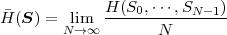
is called the entropy rate of a source S. It can be shown that the limit in (3.25) always exists for stationary sources [14]. The entropy rate (S) represents the greatest lower bound for the average codeword length per symbol that can be achieved with lossless source coding techniques,
 | (3.26) |
For iid processes, the entropy rate
is equal to the marginal entropy H(S). For stationary Markov processes, the entropy rate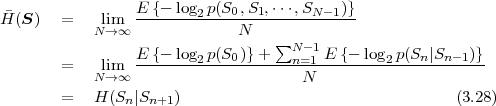
| aiak | p(ai,ak) | codewords
| |
| a0a0 | 0.58 | 1 | |
| a0a1 | 0.032 | 00001 | |
| a0a2 | 0.032 | 00010 | |
| a1a0 | 0.036 | 0010 | |
| a1a1 | 0.195 | 01 | |
| a1a2 | 0.012 | 000000 | |
| a2a0 | 0.027 | 00011 | |
| a2a1 | 0.017 | 000001 | |
| (a) | a2a2 | 0.06 | 0011 |
| N | N |
||
| 1 | 1.3556 | 3 | |
| 2 | 1.0094 | 9 | |
| 3 | 0.9150 | 27 | |
| 4 | 0.8690 | 81 | |
| 5 | 0.8462 | 243 | |
| 6 | 0.8299 | 729 | |
| 7 | 0.8153 | 2187 | |
| 8 | 0.8027 | 6561 | |
| (b) | 9 | 0.7940 | 19683 |
As an example for the design of block Huffman codes, we consider the discrete Markov process specified in Table 3.2. The entropy rate (S) for this source is 0.7331 bit per symbol. Table 3.4(a) shows a Huffman code for the joint coding of 2 symbols. The average codeword length per symbol for this code is 1.0094 bit per symbol, which is smaller than the average codeword length obtained with the Huffman code for the marginal pmf and the conditional Huffman code that we developed in sec. 3.2. As shown in Table 3.4(b), the average codeword length can be further reduced by increasing the number N of jointly coded symbols. If N approaches infinity, the average codeword length per symbol for the block Huffman code approaches the entropy rate. However, the number NC of codewords that must be stored in an encoder and decoder grows exponentially with the number N of jointly coded symbols. In practice, block Huffman codes are only used for a small number of symbols with small alphabets.
In general, the number of symbols in a message is not a multiple of the block size N. The last block of source symbols may contain less than N symbols, and, in that case, it cannot be represented with the block Huffman code. If the number of symbols in a message is known to the decoder (e.g., because it is determined by a given bitstream syntax), an encoder can send the codeword for any of the letter combinations that contain the last block of source symbols as a prefix. At the decoder side, the additionally decoded symbols are discarded. If the number of symbols that are contained in a message cannot be determined in the decoder, a special symbol for signaling the end of a message can be added to the alphabet.
3.3.2 Huffman Codes for Variable-Length Vectors
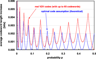
An additional degree of freedom for designing Huffman codes, or generally variable-length codes, for symbol vectors is obtained if the restriction that all codewords are assigned to symbol blocks of the same size is removed. Instead, the codewords can be assigned to sequences of a variable number of successive symbols. Such a code is also referred to as V2V code in this text. In order to construct a V2V code, a set of letter sequences with a variable number of letters is selected and a codeword is associated with each of these letter sequences. The set of letter sequences has to be chosen in a way that each message can be represented by a concatenation of the selected letter sequences. An exception is the end of a message, for which the same concepts as for block Huffman codes (see above) can be used.
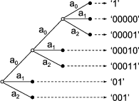
Fig. 3.3 Example for an M-ary tree representing sequences of a variable number of letters,
of the alphabet  = {a0,a1,a2}, with an associated variable length code.
Similarly as for binary codes, the set of letter sequences can be
represented by an M-ary tree as depicted in Fig. 3.3. In contrast to binary
code trees, each node has up to M descendants and each branch is labeled
with a letter of the M-ary alphabet = {a0,a1, ,aM-1}. All branches
that depart from a particular node are labeled with different letters. The
letter sequence that is represented by a particular node is given by a
concatenation of the branch labels from the root node to the particular
node. An M-ary tree is said to be a full tree if each node is either a leaf
node or has exactly M descendants.
,aM-1}. All branches
that depart from a particular node are labeled with different letters. The
letter sequence that is represented by a particular node is given by a
concatenation of the branch labels from the root node to the particular
node. An M-ary tree is said to be a full tree if each node is either a leaf
node or has exactly M descendants.
We constrain our considerations to full M-ary trees for which all leaf nodes and only the leaf nodes are associated with codewords. This restriction yields a V2V code that fulfills the necessary condition stated above and has additionally the following useful properties:
The first property implies that any message can only be represented by a single sequence of codewords. The only exception is that, if the last symbols of a message do not represent a letter sequence that is associated with a codeword, one of multiple codewords can be selected as discussed above.
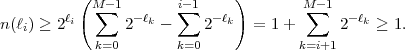
Let N denote the number of leaf nodes in a full M-ary tree
  . Each
leaf node
. Each
leaf node  k represents a sequence ak = {a0k,a1k,
 ,aNk-1k} of Nk
alphabet letters. The associated probability p(k) for coding a symbol
sequence {Sn,
,aNk-1k} of Nk
alphabet letters. The associated probability p(k) for coding a symbol
sequence {Sn, ,Sn+Nk-1} is given by
 | (3.29) |
where represents the event that the preceding symbols {S0,…,Sn-1} were
coded using a sequence of complete codewords of the V2V tree. The term
p(am|a0, ,am-1,) denotes the conditional pmf for a random variable
Sn+m given the random variables Sn to Sn+m-1 and the event .
For iid sources, the probability p(k) for a leaf node k simplifies
to
,am-1,) denotes the conditional pmf for a random variable
Sn+m given the random variables Sn to Sn+m-1 and the event .
For iid sources, the probability p(k) for a leaf node k simplifies
to
 | (3.30) |
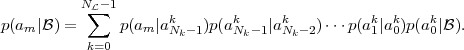
For stationary Markov sources, the probabilities p(k) are given
by
 | (3.31) |
The conditional pmfs p(am|a0, ,am-1,) are given by the structure of
the M-ary tree and the conditional pmfs p(am|a0,
,am-1,) are given by the structure of
the M-ary tree and the conditional pmfs p(am|a0, ,am-1) for the
random variables Sn+m assuming the preceding random variables Sn to
Sn+m-1.
,am-1) for the
random variables Sn+m assuming the preceding random variables Sn to
Sn+m-1.
As an example, we show how the pmf p(a|) = P(Sn = a|) that is
conditioned on the event can be determined for Markov sources. In this
case, the probability p(am|) = P(Sn = am|) that a codeword is assigned
to a letter sequence that starts with a particular letter am of the alphabet
= {a0,a1, ,aM-1} is given by
 | (3.32) |
These M equations form a homogeneous linear equation system that has
one set of non-trivial solutions p(a|) = κ ⋅{x0,x1, ,xM-1}. The scale
factor κ and thus the pmf p(a|) can be uniquely determined by using the
constraint ∑
m=0M-1p(am|) = 1.
,xM-1}. The scale
factor κ and thus the pmf p(a|) can be uniquely determined by using the
constraint ∑
m=0M-1p(am|) = 1.
After the conditional pmfs p(am|a0, ,am-1,) have been determined,
the pmf p() for the leaf nodes can be calculated. An optimal prefix code
for the selected set of letter sequences, which is represented by the leaf
nodes of a full M-ary tree , can be designed using the Huffman algorithm
for the pmf p(). Each leaf node k is associated with a codeword of ℓk
bits. The average codeword length per symbol is given by the ratio of the
average codeword length per letter sequence and the average number of
letters per letter sequence,
,am-1,) have been determined,
the pmf p() for the leaf nodes can be calculated. An optimal prefix code
for the selected set of letter sequences, which is represented by the leaf
nodes of a full M-ary tree , can be designed using the Huffman algorithm
for the pmf p(). Each leaf node k is associated with a codeword of ℓk
bits. The average codeword length per symbol is given by the ratio of the
average codeword length per letter sequence and the average number of
letters per letter sequence,
 | (3.33) |
For selecting the set of letter sequences or the full M-ary tree , we
assume that the set of applicable V2V codes for an application is given by
parameters such as the maximum number of codewords (number of leaf
nodes). Given such a finite set of full M-ary trees, we can select the full
M-ary tree , for which the Huffman code yields the smallest average
codeword length per symbol .
| ak | p(  k) k) | codewords
| |
| a0a0 | 0.5799 | 1 | |
| a0a1 | 0.0322 | 00001 | |
| a0a2 | 0.0322 | 00010 | |
| a1a0 | 0.0277 | 00011 | |
| a1a1a0 | 0.0222 | 000001 | |
| a1a1a1 | 0.1183 | 001 | |
| a1a1a2 | 0.0074 | 0000000 | |
| a1a2 | 0.0093 | 0000001 | |
| (a) | a2 | 0.1708 | 01 |
| N | ||
| 5 | 1.1784 | |
| 7 | 1.0551 | |
| 9 | 1.0049 | |
| 11 | 0.9733 | |
| 13 | 0.9412 | |
| 15 | 0.9293 | |
| 17 | 0.9074 | |
| 19 | 0.8980 | |
| (b) | 21 | 0.8891 |
= 9 codewords; (b) Average codeword lengths depending on the number of
codewords N.
As an example for the design of a V2V Huffman code, we again consider the stationary discrete Markov source specified in Table 3.2. Table 3.5(a) shows a V2V code that minimizes the average codeword length per symbol among all V2V codes with up to 9 codewords. The average codeword length is 1.0049 bit per symbol, which is about 0.4% smaller than the average codeword length for the block Huffman code with the same number of codewords. As indicated in Table 3.5(b), when increasing the number of codewords, the average codeword length for V2V codes usually decreases faster as for block Huffman codes. The V2V code with 17 codewords has already an average codeword length that is smaller than that of the block Huffman code with 27 codewords.
An application example of V2V codes is the run-level coding of transform coefficients in MPEG-2 Video [39]. An often used variation of V2V codes is called run-length coding. In run-length coding, the number of successive occurrences of a particular alphabet letter, referred to as run, is transmitted using a variable-length code. In some applications, only runs for the most probable alphabet letter (including runs equal to 0) are transmitted and are always followed by a codeword for one of the remaining alphabet letters. In other applications, the codeword for a run is followed by a codeword specifying the alphabet letter, or vice versa. V2V codes are particularly attractive for binary iid sources. As we will show in sec. 3.5, a universal lossless source coding concept can be designed using V2V codes for binary iid sources in connection with the concepts of binarization and probability interval partitioning.
3.4 Elias Coding and Arithmetic Coding
Huffman codes achieve the minimum average codeword length among all uniquely decodable codes that assign a separate codeword to each element of a given set of alphabet letters or letter sequences. However, if the pmf for a symbol alphabet contains a probability mass that is close to one, a Huffman code with an average codeword length close to the entropy rate can only be constructed if a large number of symbols is coded jointly. Such a block Huffman code does however require a huge codeword table and is thus impractical for real applications. Additionally, a Huffman code for fixed- or variable-length vectors is not applicable or at least very inefficient for symbol sequences in which symbols with different alphabets and pmfs are irregularly interleaved, as it is often found in image and video coding applications, where the order of symbols is determined by a sophisticated syntax.
Furthermore, the adaptation of Huffman codes to sources with unknown or varying statistical properties is usually considered as too complex for real-time applications. It is desirable to develop a code construction method that is capable of achieving an average codeword length close to the entropy rate, but also provides a simple mechanism for dealing with nonstationary sources and is characterized by a complexity that increases linearly with the number of coded symbols.
The popular method of arithmetic coding provides these properties. The initial idea is attributed to P. Elias (as reported in [1]) and is also referred to as Elias coding. The first practical arithmetic coding schemes have been published by Pasco [61] and Rissanen [63]. In the following, we first present the basic concept of Elias coding and continue with highlighting some aspects of practical implementations. For further details, the interested reader is referred to [78], [58] and [65].
We consider the coding of symbol sequences s = {s0,s1,…,sN-1} that
represent realizations of a sequence of discrete random variables
S = {S0,S1,…,SN-1}. The number N of symbols is assumed to be
known to both encoder and decoder. Each random variable Sn can be
characterized by a distinct Mn-ary alphabet n. The statistical properties
of the sequence of random variables S are completely described by the joint
pmf

A symbol sequence sa = {s0a,s1a, ,sN-1a} is considered to be less than
another symbol sequence sb = {s0b,s1b,
,sN-1a} is considered to be less than
another symbol sequence sb = {s0b,s1b, ,sN-1b} if and only if there
exists an integer n, with 0 ≤ n ≤ N - 1, so that
,sN-1b} if and only if there
exists an integer n, with 0 ≤ n ≤ N - 1, so that
 | (3.34) |
Using this definition, the probability mass of a particular symbol sequence s can written as
 | (3.35) |
This expression indicates that a symbol sequence s can be represented by
an interval  N between two successive values of the cumulative
probability mass function P(S ≤ s). The corresponding mapping of
a symbol sequence s to a half-open interval N ⊂ [0,1) is given
by
N between two successive values of the cumulative
probability mass function P(S ≤ s). The corresponding mapping of
a symbol sequence s to a half-open interval N ⊂ [0,1) is given
by
 | (3.36) |
The interval width WN is equal to the probability P(S = s) of the
associated symbol sequence s. In addition, the intervals for different
realizations of the random vector S are always disjoint. This can be shown
by considering two symbol sequences sa and sb, with sa < sb. The lower
interval boundary LNb of the interval N(sb),
 N(sa). Consequently, an N-symbol sequence s can be
uniquely represented by any real number v ∈N, which can be written as
binary fraction with K bits after the binary point,
N(sa). Consequently, an N-symbol sequence s can be
uniquely represented by any real number v ∈N, which can be written as
binary fraction with K bits after the binary point,
 | (3.38) |
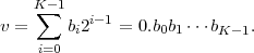
In order to identify the symbol sequence s we only need to transmit the bit
sequence b = {b0,b1, ,bK-1}. The Elias code for the sequence of random
variables S is given by the assignment of bit sequences b to the N-symbol
sequences s.
,bK-1}. The Elias code for the sequence of random
variables S is given by the assignment of bit sequences b to the N-symbol
sequences s.
For obtaining codewords that are as short as possible, we should choose the real numbers v that can be represented with the minimum amount of bits. The distance between successive binary fractions with K bits after the binary point is 2-K. In order to guarantee that any binary fraction with K bits after the decimal point falls in an interval of size WN, we need K ≥-log 2WN bits. Consequently, we choose
 | (3.39) |
where ⌈x⌉ represents the smallest integer greater than or equal to x. The binary fraction v, and thus the bit sequence b, is determined by
 | (3.40) |
An application of the inequalities ⌈x⌉≥ x and ⌈x⌉ < x + 1 to (3.40) and (3.39) yields
 | (3.41) |
which proves that the selected binary fraction v always lies inside the
interval N. The Elias code obtained by choosing K = ⌈-log 2WN⌉
associates each N-symbol sequence s with a distinct codeword b.
An important property of the Elias code is that the codewords can be
iteratively constructed. For deriving the iteration rules, we consider
sub-sequences s(n) = {s0,s1, ,sn-1} that consist of the first n symbols, with
1 ≤ n ≤ N, of the symbol sequence s. Each of these sub-sequences s(n) can
be treated in the same way as the symbol sequence s. Given the interval
width Wn for the sub-sequence s(n) = {s0,s1,…,sn-1}, the interval
width Wn+1 for the sub-sequence s(n+1) = {s(n),sn} can be derived by
,sn-1} that consist of the first n symbols, with
1 ≤ n ≤ N, of the symbol sequence s. Each of these sub-sequences s(n) can
be treated in the same way as the symbol sequence s. Given the interval
width Wn for the sub-sequence s(n) = {s0,s1,…,sn-1}, the interval
width Wn+1 for the sub-sequence s(n+1) = {s(n),sn} can be derived by
 ) being the conditional probability mass function
P
) being the conditional probability mass function
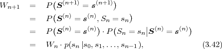
P . Similarly, the iteration rule
for the lower interval border Ln is given by where c(sn
. Similarly, the iteration rule
for the lower interval border Ln is given by where c(sn ) represents a cumulative probability mass
function (cmf) and is given by
) represents a cumulative probability mass
function (cmf) and is given by
 | (3.44) |
By setting W0 = 1 and L0 = 0, the iteration rules (3.42) and (3.43) can also be used for calculating the interval width and lower interval border of the first sub-sequence s(1) = {s0}. Equation (3.43) directly implies Ln+1 ≥ Ln. By combining (3.43) and (3.42), we also obtain
 n+1 for a symbol sequence s(n+1) is nested inside
the interval n for the symbol sequence s(n) that excludes the last
symbol sn.
n+1 for a symbol sequence s(n+1) is nested inside
the interval n for the symbol sequence s(n) that excludes the last
symbol sn.
The iteration rules have been derived for the general case of dependent and differently distributed random variables Sn. For iid processes and Markov processes, the general conditional pmf in (3.42) and (3.44) can be replaced with the marginal pmf p(sn) = P(Sn = sn) and the conditional pmf p(sn|sn-1) = P(Sn = sn|Sn-1 = sn-1), respectively.
As an example, we consider the iid process in Table 3.6. Beside the pmf p(a) and cmf c(a), the table also specifies a Huffman code. Suppose we intend to transmit the symbol sequence s =‘CABAC’. If we use the Huffman code, the transmitted bit sequence would be b =‘10001001’. The iterative code construction process for the Elias coding is illustrated in Table 3.7. The constructed codeword is identical to the codeword that is obtained with the Huffman code. Note that the codewords of an Elias code have only the same number of bits as the Huffman code if all probability masses are integer powers of 1∕2 as in our example.
| s
0=‘C’ | s1=‘A’ | s2=‘B’ |
| W1 = W0 ⋅p(‘C’) | W2 = W1 ⋅p(‘A’) | W3 = W2 ⋅p(‘B’) |
| = 1 ⋅ 2-1 = 2-1 | = 2-1 ⋅ 2-2 = 2-3 | = 2-3 ⋅ 2-2 = 2-5 |
| = (0.1)b | = (0.001)b | = (0.00001)b |
| L1 = L0 + W0 ⋅c(‘C’) | L2 = L1 + W1 ⋅c(‘A’) | L3 = L2 + W2 ⋅c(‘B’) |
| = L0 + 1 ⋅ 2-1 | = L 1 + 2-1 ⋅ 0 | = L 2 + 2-3 ⋅ 2-2 |
| = 2-1 | = 2-1 | = 2-1 + 2-5 |
| = (0.1)b | = (0.100)b | = (0.10001)b |
| s
3=‘A’ | s4=‘C’ | termination |
| W4 = W3 ⋅p(‘A’) | W5 = W4 ⋅p(‘C’) | K = ⌈- log 2W5⌉ = 8 |
| = 2-5 ⋅ 2-2 = 2-7 | = 2-7 ⋅ 2-1 = 2-8 | |
| = (0.0000001)b | = (0.00000001)b | v =  L52K L52K 2-K 2-K |
| L4 = L3 + W3 ⋅c(‘A’) | L5 = L4 + W4 ⋅c(‘C’) | = 2-1 + 2-5 + 2-8 |
| = L3 + 2-5 ⋅ 0 | = L 4 + 2-7 ⋅ 2-1 | |
| = 2-1 + 2-5 | = 2-1 + 2-5 + 2-8 | b = ‘10001001′ |
| = (0.1000100)b | = (0.10001001)b | |
Based on the derived iteration rules, we state an iterative encoding and
decoding algorithm for Elias codes. The algorithms are specified for the
general case using multiple symbol alphabets and conditional pmfs and
cmfs. For stationary processes, all alphabets n can be replaced by a single
alphabet . For iid sources, Markov sources, and other simple source
models, the conditional pmfs p(sn|s0, ,sn-1) and cmfs c(sn|s0,
 ,sn-1)
can be simplified as discussed above.
,sn-1)
can be simplified as discussed above.
Encoding algorithm:
 ,sN-1} of N symbols.
 ,N - 1, determine the interval n+1 by
Decoding algorithm:
 ,bK-1} of KN bits.
 ,N - 1, do the following:
n, determine the interval n+1(ai) by
,N - 1, do the following:
n, determine the interval n+1(ai) by
 n for which v ∈n+1(ai),
Since the iterative interval refinement is the same at encoder and
decoder side, Elias coding provides a simple mechanism for the adaptation
to sources with unknown or nonstationary statistical properties.
Conceptually, for each source symbol sn, the pmf p(sn|s0, ,sn-1) can be
simultaneously estimated at encoder and decoder side based on the already
coded symbols s0 to sn-1. For this purpose, a source can often be modeled
as a process with independent random variables or as a Markov
process. For the simple model of independent random variables, the
pmf p(sn) for a particular symbol sn can be approximated by the
relative frequencies of the alphabet letters inside the sequence of
the preceding NW coded symbols. The chosen interval size NW
adjusts the trade-off between a fast adaptation and an accurate
probability estimation. The same approach can also be applied for
high-order probability models as the Markov model. In this case, the
conditional pmf is approximated by the corresponding relative conditional
frequencies.
,sn-1) can be
simultaneously estimated at encoder and decoder side based on the already
coded symbols s0 to sn-1. For this purpose, a source can often be modeled
as a process with independent random variables or as a Markov
process. For the simple model of independent random variables, the
pmf p(sn) for a particular symbol sn can be approximated by the
relative frequencies of the alphabet letters inside the sequence of
the preceding NW coded symbols. The chosen interval size NW
adjusts the trade-off between a fast adaptation and an accurate
probability estimation. The same approach can also be applied for
high-order probability models as the Markov model. In this case, the
conditional pmf is approximated by the corresponding relative conditional
frequencies.
The average codeword length per symbol for the Elias code is given by
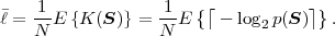 | (3.46) |
By applying the inequalities ⌈x⌉≥ x and ⌈x⌉ < x + 1, we obtain
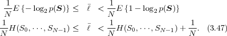
It should be noted that the Elias code is not guaranteed to be prefix free, i.e., a codeword for a particular symbol sequence may be a prefix of the codeword for any other symbol sequence. Hence, the Elias code as described above can only be used if the length of the codeword is known at the decoder side5. A prefix-free Elias code can be constructed if the lengths of all codewords are increased by one, i.e., by choosing
 | (3.48) |
The Elias code has several desirable properties, but it is still impractical, since the precision that is required for representing the interval widths and lower interval boundaries grows without bound for long symbol sequences. The widely-used approach of arithmetic coding is a variant of Elias coding that can be implemented with fixed-precision integer arithmetic.
For the following considerations, we assume that the probability masses
p(sn|s0, ,sn-1) are given with a fixed number V of binary digit after the
binary point. We will omit the conditions “s0,
,sn-1) are given with a fixed number V of binary digit after the
binary point. We will omit the conditions “s0, ,sn-1” and represent the
pmfs p(a) and cmfs c(a) by
,sn-1” and represent the
pmfs p(a) and cmfs c(a) by
 | (3.49) |
where pV (a) and cV (a) are V -bit positive integers.
The key observation for designing arithmetic coding schemes is that the Elias code remains decodable if the interval width Wn+1 satisfies
 | (3.50) |
This guarantees that the interval n+1 is always nested inside the interval
n. Equation (3.43) implies Ln+1 ≥ Ln, and by combining (3.43) with the
inequality (3.50), we obtain
![Ln+1 + Wn+1 ≤ Ln + Wn ⋅[c(sn)+ p(sn)] ≤ Ln + Wn.](VBpart1171x.png) | (3.51) |
Hence, we can represent the interval width Wn with a fixed number of precision bits if we round it toward zero in each iteration step.
Let the interval width Wn be represented by a U-bit integer An and an integer zn ≥ U according to
 | (3.52) |
We restrict An to the range
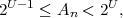 | (3.53) |
so that the Wn is represented with a maximum precision of U bits. In order to suitably approximate W0 = 1, the values of A0 and z0 are set equal to 2U - 1 and U, respectively. The interval refinement can then be specified by
where yn is a bit shift parameter with 0 ≤ yn ≤ V . These iteration rules guarantee that (3.50) is fulfilled. It should also be noted that the operation ⌊x ⋅ 2-y⌋ specifies a simple right shift of the binary representation of x by y binary digits. To fulfill the constraint in (3.53), the bit shift parameter yn has to be chosen according to
 | (3.56) |
The value of yn can be determined by a series of comparison operations.
Given the fixed-precision representation of the interval width Wn, we investigate the impact on the lower interval boundary Ln. The binary representation of the product
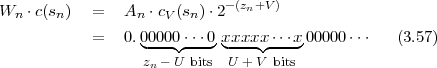
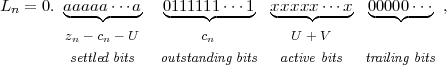 | (3.58) |
can be classified into four categories. The trailing bits that follow the
(zn + V )-th bit after the binary point are equal to 0, but may be modified
by following interval updates. The preceding U + V bits are directly
modified by the update Ln+1 = Ln + Wnc(sn) and are referred to as
active bits. The active bits are preceded by a sequence of zero or
more 1-bits and a leading 0-bit (if present). These cn bits are called
outstanding bits and may be modified by a carry from the active bits.
The zn -cn -U bits after the binary point, which are referred to
as settled bits, are not modified in any following interval update.
Furthermore, these bits cannot be modified by the rounding operation
that generates the final codeword, since all intervals n+k, with
k > 0, are nested inside the interval n and the binary representation
of the interval width Wn = An2-zn also consists of zn - U 0-bits
after the binary point. And since the number of bits in the final
codeword,
 | (3.59) |
is always greater than or equal to the number of settled bits, the settled bits can be transmitted as soon as they have become settled. Hence, in order to represent the lower interval boundary Ln, it is sufficient to store the U + V active bits and a counter for the number of 1-bits that precede the active bits.
For the decoding of a particular symbol sn it has to be determined whether the binary fraction v in (3.40) that is represented by the transmitted codeword falls inside the interval Wn+1(ai) for an alphabet letter ai. Given the described fixed-precision interval refinement, it is sufficient to compare the cn+1 outstanding bits and the U + V active bits of the lower interval boundary Ln+1 with the corresponding bits of the transmitted codeword and the upper interval boundary Ln+1 + Wn+1.
It should be noted that the number of outstanding bits can become arbitrarily large. In order to force an output of bits, the encoder can insert a 0-bit if it detects a sequence of a particular number of 1-bits. The decoder can identify the additionally inserted bit and interpret it as extra carry information. This technique is for example used in the MQ-coder [72] of JPEG 2000 [41].
In comparison to Elias coding, the usage of the presented fixed
precision approximation increases the codeword length for coding
a symbol sequence s = {s0,s1, ,sN-1}. Given WN for n = N
in (3.52), the excess rate of arithmetic coding over Elias coding is given
by
,sN-1}. Given WN for n = N
in (3.52), the excess rate of arithmetic coding over Elias coding is given
by
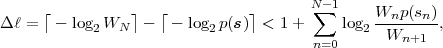 | (3.60) |
where we used the inequalities ⌈x⌉ < x + 1 and ⌈x⌉≥ x to derive the upper bound on the right side. We shall further take into account that we may have to approximate the real pmfs p(a) in order to represent the probability masses as multiples of 2-V . Let q(a) represent an approximated pmf that is used for arithmetic coding and let pmin denote the minimum probability mass of the corresponding real pmf p(a). The pmf approximation can always be done in a way that the difference p(a) - q(a) is less than 2-V , which gives
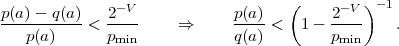 | (3.61) |
An application of the inequality ⌊x⌋ > x - 1 to the interval refinement (3.54) with the approximated pmf q(a) yields
By using the relationship Wn+1 ≥ 2U-1-zn+1, which is a direct consequence of (3.53), we obtain
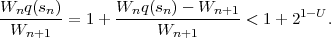 | (3.63) |
Inserting the expressions (3.61) and (3.63) into (3.60) yields an upper bound for the increase in codeword length per symbol,
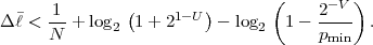 | (3.64) |
If we consider, for example, the coding of N = 1000 symbols with U = 12, V = 16, and pmin = 0.02, the increase in codeword length in relation to Elias coding is guaranteed to be less than 0.003 bit per symbol.
Arithmetic coding with binary symbol alphabets is referred to as binary arithmetic coding. It is the most popular type of arithmetic coding in image and video coding applications. The main reason for using binary arithmetic coding is its reduced complexity. It is particularly advantageous for adaptive coding, since the rather complex estimation of M-ary pmfs can be replaced by the simpler estimation of binary pmfs. Well-known examples of efficient binary arithmetic coding schemes that are used in image and video coding are the MQ-coder [72] in the picture coding standard JPEG 2000 [41] and the M-coder [55] in the video coding standard H.264/AVC [36].
In general, a symbol sequence s = {s0,s1, ,sN-1} has to be first
converted into a sequence c = {c0,c1,
,sN-1} has to be first
converted into a sequence c = {c0,c1, ,cB-1} of binary symbols, before
binary arithmetic coding can be applied. This conversion process is often
referred to as binarization and the elements of the resulting binary
sequences c are also called bins. The number B of bins in a sequence c can
depend on the actual source symbol sequence s. Hence, the bin
sequences c can be interpreted as realizations of a variable-length sequence
of binary random variables C = {C0,C1,
,cB-1} of binary symbols, before
binary arithmetic coding can be applied. This conversion process is often
referred to as binarization and the elements of the resulting binary
sequences c are also called bins. The number B of bins in a sequence c can
depend on the actual source symbol sequence s. Hence, the bin
sequences c can be interpreted as realizations of a variable-length sequence
of binary random variables C = {C0,C1, ,CB-1}.
Conceptually, the binarization mapping S → C represents a lossless
coding step and any lossless source code could be applied for this purpose.
It is, however, only important that the used lossless source code is uniquely
decodable. The average codeword length that is achieved by the
binarization mapping does not have any impact on the efficiency of binary
arithmetic coding, since the block entropy for the sequence of random
variables S = {S0,S1, ,SN-1},
 |
is equal to entropy of the variable-length binary random vector
C = {C0,C1, ,CB-1}. The actual compression is achieved by the
arithmetic coding. The above result also shows that binary arithmetic
coding can provide the same coding efficiency as M-ary arithmetic coding,
if the influence of the finite precision arithmetic is negligible.
,CB-1}. The actual compression is achieved by the
arithmetic coding. The above result also shows that binary arithmetic
coding can provide the same coding efficiency as M-ary arithmetic coding,
if the influence of the finite precision arithmetic is negligible.
In practice, the binarization is usually done with very simple prefix codes for the random variables Sn. As we assume that the order of different random variables is known to both, encoder and decoder, different prefix codes can be used for each random variable without impacting unique decodability. A typical example for a binarization mapping, which is called truncated unary binarization, is illustrated in Table 3.8.
The binary pmfs for the random variables Ci can be directly derived from the pmfs of the random variables Sn. For the example in Table 3.8, the binary pmf {P(Ci = 0),1 - P(Ci = 0)} for a random variable Ci is given by
 | (3.65) |
where we omitted the condition for the binary pmf. For coding nonstationary sources, it is usually preferable to directly estimate the marginal or conditional pmf’s for the binary random variables instead of the pmf’s for the source signal.
3.5 Probability Interval Partitioning Entropy Coding
For a some applications, arithmetic coding is still considered as too complex. As a less-complex alternative, a lossless coding scheme called probability interval partitioning entropy (PIPE) coding has been recently proposed [54]. It combines concepts from binary arithmetic coding and Huffman coding for variable-length vectors with a quantization of the binary probability interval.
A block diagram of the PIPE coding structure is shown in Fig. 3.4. It is
assumed that the input symbol sequences s = {s0,s1, ,sN-1} represent
realizations of a sequence S = {S0,S1,
,sN-1} represent
realizations of a sequence S = {S0,S1, ,SN-1} of random variables.
Each random variable can be characterized by a distinct alphabet n. The
number N of source symbols is assumed to be known to encoder
and decoder. Similarly as for binary arithmetic coding, a symbol
sequence s = {s0,s1,
,SN-1} of random variables.
Each random variable can be characterized by a distinct alphabet n. The
number N of source symbols is assumed to be known to encoder
and decoder. Similarly as for binary arithmetic coding, a symbol
sequence s = {s0,s1, ,sN-1} is first converted into a sequence
c = {c0,c1,
,sN-1} is first converted into a sequence
c = {c0,c1, ,cB-1} of B binary symbols (bins). Each bin ci can
be considered as a realization of a corresponding random variable
Ci and is associated with a pmf. The binary pmf is given by the
probability P(Ci = 0), which is known to encoder and decoder. Note that
the conditional dependencies have been omitted in order to simplify the
description.
,cB-1} of B binary symbols (bins). Each bin ci can
be considered as a realization of a corresponding random variable
Ci and is associated with a pmf. The binary pmf is given by the
probability P(Ci = 0), which is known to encoder and decoder. Note that
the conditional dependencies have been omitted in order to simplify the
description.
The key observation for designing a low-complexity alternative to binary
arithmetic coding is that an appropriate quantization of the binary
probability interval has only a minor impact on the coding efficiency. This
is employed by partitioning the binary probability interval into a small
number U of half-open intervals k = (pk,pk+1], with 0 ≤ k < U. Each bin
ci is assigned to the interval k for which pk < P(Ci = 0) ≤ pk+1. As
a result, the bin sequence c is decomposed into U bin sequences
uk = {u0k,u1k,…}, with 0 ≤ k < U. For the purpose of coding, each of the
bin sequences uk can be treated as a realization of a binary iid process with
a pmf {p k,1 - pk}, where pk denotes a representative probability for
an interval k, and can be efficiently coded with a V2V code as
described in sec. 3.3. The resulting U codeword sequences bk are finally
multiplexed in order to produce a data packet for the symbol sequence
s.
k,1 - pk}, where pk denotes a representative probability for
an interval k, and can be efficiently coded with a V2V code as
described in sec. 3.3. The resulting U codeword sequences bk are finally
multiplexed in order to produce a data packet for the symbol sequence
s.
Given the U probability intervals k = (pk,pk+1] and corresponding
V2V codes, the PIPE coding process can be summarized as follows:
k in the same order as in the bin sequence c.
The binarization process is the same as for binary arithmetic coding
described in sec. 3.4. Typically, each symbol sn of the input symbol
sequence s = {s0,s1, ,sN-1} is converted into a sequence cn of a
variable number of bins using a simple prefix code and these bin
sequences cn are concatenated to produce the bin sequence c that uniquely
represents the input symbol sequence s. Here, a distinct prefix code can be
used for each random variable Sn. Given the prefix codes, the conditional
binary pmfs
,sN-1} is converted into a sequence cn of a
variable number of bins using a simple prefix code and these bin
sequences cn are concatenated to produce the bin sequence c that uniquely
represents the input symbol sequence s. Here, a distinct prefix code can be
used for each random variable Sn. Given the prefix codes, the conditional
binary pmfs

can be directly derived based on the conditional pmfs for the random variables Sn. The binary pmfs can either be fixed or they can be simultaneously estimated at encoder and decoder side6. In order to simplify the following description, we omit the conditional dependencies and specify the binary pmf for the i-th bin by the probability P(Ci = 0).
For the purpose of binary coding, it is preferable to use bin sequences c for which all probabilities P(Ci = 0) are less than or equal to 0.5. This property can be ensured by inverting a bin value ci if the associated probability P(Ci = 0) is greater than 0.5. The inverse operation can be done at the decoder side, so that the unique decodability of a symbol sequence s from the associated bin sequence c is not influenced. For PIPE coding, we assume that this additional operation is done during the binarization and that all bins ci of a bin sequence c are associated with probabilities P(Ci = 0) ≤ 0.5.
| Ci(Sn) | C0(Sn) | C1(Sn) |
| P(Ci(Sn) = 0|Sn-1 = a0) | 0.10 | 0.50 |
| P(Ci(Sn) = 0|Sn-1 = a1) | 0.15 | 1/17 |
| P(Ci(Sn) = 0|Sn-1 = a2) | 0.25 | 0.20 |
As an example, we consider the binarization for the stationary Markov source in specified in Table 3.2. If the truncated unary binarization given in Table 3.8 is used and all bins with probabilities P(Ci = 0) greater than 0.5 are inverted, we obtain the bin probabilities given in Table 3.9. Ci(Sn) denotes the random variable that corresponds to the i-th bin inside the bin sequences for the random variable Sn.
The half-open probability interval (0,0.5], which includes all possible bin
probabilities P(Ci = 0), is partitioned into U intervals k = (pk,pk+1]. This
set of intervals is characterized by U - 1 interval borders pk with
k = 1, ,U - 1. Without loss of generality, we assume pk < pk+1. The
outer interval borders are fixed and given by p0 = 0 and pU = 0.5. Given
the interval boundaries, the sequence of bins c is decomposed into U
separate bin sequences uk = (u0k,u1k,
,U - 1. Without loss of generality, we assume pk < pk+1. The
outer interval borders are fixed and given by p0 = 0 and pU = 0.5. Given
the interval boundaries, the sequence of bins c is decomposed into U
separate bin sequences uk = (u0k,u1k, ), where each bin sequence uk
contains the bins ci with P(Ci = 0) ∈k. Each bin sequence uk is coded
with a binary coder that is optimized for a representative probability pk
for the interval k.
), where each bin sequence uk
contains the bins ci with P(Ci = 0) ∈k. Each bin sequence uk is coded
with a binary coder that is optimized for a representative probability pk
for the interval k.
For analyzing the impact of the probability interval partitioning, we
assume that we can design a lossless code for binary iid processes that
achieves the entropy limit. The average codeword length ℓb(p,pk) for
coding a bin ci with the probability p = P(Ci = 0) using an optimal code
for the representative probability pk is given by
 | (3.66) |
When we further assume that the relative frequencies of the bin
probabilities p inside a bin sequence c are given by the pdf f(p), the
average codeword length per bin b for a given set of U intervals k with
representative probabilities pk can then be written as
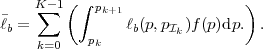 | (3.67) |
Minimization with respect to the interval boundaries pk and representative
probabilities pk yields the equation system,
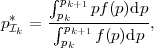 | (3.68) |
 | (3.69) |
Given the pdf f(p) and the number of intervals U, the interval partitioning
can be derived by an iterative algorithm that alternately updates the
interval borders pk and interval representatives pk. As an example,
Fig. 3.5 shows the probability interval partitioning for a uniform
distribution f(p) of the bin probabilities and U = 4 intervals. As can be
seen, the probability interval partitioning leads to a piecewise linear
approximation ℓb(p,pk)|k of the binary entropy function H(p).
Fig. 3.5 Example for the partitioning of the probability interval (0, 0.5] into 4 intervals assuming a uniform distribution of the bin probabilities p = P(Ci = 0).
The increase of the average codeword length per bin is given by
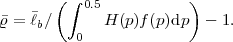 | (3.70) |
Table 3.10 lists the increases in average codeword length per bin for a uniform and a linear increasing (f(p) = 8p) distribution of the bin probabilities for selected numbers U of intervals.
| U | 1 | 2 | 4 | 8 | 12 | 16 |
| uni [%] | 12.47 | 3.67 | 1.01 | 0.27 | 0.12 | 0.07 |
| lin [%] | 5.68 | 1.77 | 0.50 | 0.14 | 0.06 | 0.04 |
We now consider the probability interval partitioning for the Markov source specified in Table 3.2. As shown in Table 3.9, the binarization described above led to 6 different bin probabilities. For the truncated unary binarization of a Markov source, the relative frequency h(pij) that a bin with probability pij = P(Ci(Sn)|Sn-1 = aj) occurs inside the bin sequence c is equal to
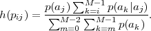 | (3.71) |
The distribution of the bin probabilities is given by

interval  k = (pk,pk+1] k = (pk,pk+1] | representative p k k |
| 0 = (0, 0.1326] | 0.09 |
| 1 = (0.1326, 0.3294] | 0.1848 |
| 2 = (0.3294, 0.5] | 0.5000 |
For the purpose of binary coding, a bin sequence uk for the probability
interval k can be treated as a realization of a binary iid process
with a pmf {pk,1 - pk}. The statistical dependencies between the
bins have already been exploited by associating each bin ci with a
probability P(Ci = 0) that depends on previously coded bins or symbols
according to the employed probability modeling. The V2V codes
described in sec. 3.3 are simple but very efficient lossless source
codes for binary iid processes Uk = {Unk}. Using these codes, a
variable number of bins is mapped to a variable-length codeword.
By considering a sufficiently large number of tables entries, these
codes can achieve an average codeword length close to the entropy
rate (Uk) = H(Unk).
| p
0 = 0.09 | p 1 = 0.1848 | p
2 = 0.5 | |||
| 0 = 0.4394,ϱ0 = 0.69% | 1 = 0.6934,ϱ1 = 0.42% | 2 = 1,ϱ2 = 0%
| |||
| bin sequence | codeword | bin sequence | codeword | bin sequence | codeword |
| ′1111111′ | ′1′ | ′111′ | ′1′ | ′1′ | ′1′ |
| ′0′ | ′011′ | ′110′ | ′001′ | ′0′ | ′0′ |
| ′10′ | ′0000′ | ′011′ | ′010′ | ||
| ′110′ | ′0001′ | ′1011′ | ′011′ | ||
| ′1110′ | ′0010′ | ′00′ | ′00000′ | ||
| ′11110′ | ′0011′ | ′100′ | ′00001′ | ||
| ′111110′ | ′0100′ | ′010′ | ′00010′ | ||
| ′1111110′ | ′0101′ | ′1010′ | ′00011′ | ||
k of the probability interval partitioning specified in Table 3.11.
As an example, Table 3.12 shows V2V codes for the interval
representatives pk of the probability interval partitioning given in
Table 3.11. These codes achieve the minimum average codeword length
per bin among all V2V codes with up to 8 codewords. The table
additionally lists the average codeword lengths per bin k and the
corresponding redundancies ϱk =  k -(Uk)
 ∕(Uk). The code
redundancies could be further decreased if V2V codes with more
than 8 codewords are considered. When we assume that the number
of N of symbols approaches infinity, the average codeword length
per symbol for the applied truncated unary binarization is given
by
∕(Uk). The code
redundancies could be further decreased if V2V codes with more
than 8 codewords are considered. When we assume that the number
of N of symbols approaches infinity, the average codeword length
per symbol for the applied truncated unary binarization is given
by
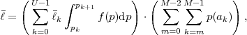 | (3.72) |
where the first term represents the average codeword length per bin for the bin sequence c and the second term is the bin-to-symbol ratio. For our simple example, the average codeword length for the PIPE coding is = 0.7432 bit per symbol. It is only 1.37% larger than the entropy rate and significantly smaller than the average codeword length for the scalar, conditional, and block Huffman codes that we have developed in sec. 3.2 and sec. 3.3.
In general, the average codeword length per symbol can be further
decreased if the V2V codes and the probability interval partitioning are
jointly optimized. This can be achieved by an iterative algorithm that
alternately optimizes the interval representatives pk, the V2V codes for
the interval representatives, and the interval boundaries pk. Each
codeword entry m of a binary V2V code  k is characterized by the
number xm of 0-bins, the number ym of 1-bins, and the length ℓm of
the codeword. As can be concluded from the description of V2V
codes in sec. 3.3, the average codeword length for coding a bin ci
with a probability p = P(Ci = 0) using a V2V code k is given
by
k is characterized by the
number xm of 0-bins, the number ym of 1-bins, and the length ℓm of
the codeword. As can be concluded from the description of V2V
codes in sec. 3.3, the average codeword length for coding a bin ci
with a probability p = P(Ci = 0) using a V2V code k is given
by
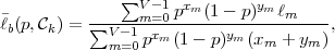 | (3.73) |
where V denotes the number of codeword entries. Hence, an optimal
interval border pk is given by the intersection point of the functions
b(p,k-1) and b(p,k) for the V2V codes of the neighboring intervals.
Fig. 3.6 Difference between the average codeword length and the binary entropy function H(p) for a probability interval partitioning into U = 12 intervals assuming optimal binary codes and a real design with V2V codes of up to 65 codeword entries. The distribution of bin probabilities is assumed to be uniform.
As an example, we jointly derived the partitioning into U = 12
probability intervals and corresponding V2V codes with up to 65 codeword
entries for a uniform distribution of bin probabilities. Fig. 3.6 shows the
difference between the average codeword length per bin and the
binary entropy function H(p) for this design and a theoretically
optimal probability interval partitioning assuming optimal binary
codes with k = H(pk). The overall redundancy with respect to the
entropy limit is 0.24% for the jointly optimized design and 0.12%
for the probability interval partitioning assuming optimal binary
codes.
The U codeword sequences bk that are generated by the different binary encoders for a set of source symbols (e.g., a slice of a video picture) can be written to different partitions of a data packet. This enables a parallelization of the bin encoding and decoding process. At the encoder side, each sub-sequence uk is written to a different buffer and the actual binary encoding can be done in parallel. At the decoder side, the U codeword sequences bk can be decoded in parallel and the resulting bin sequences uk can be stored in separate bin buffers. The remaining entropy decoding process can then be designed in a way that it simply reads bins from the corresponding U bin buffers.
The separate transmission of the codeword streams requires the
signaling of partitioning information. Furthermore, parallelized entropy
coding is often not required for small data packets. In such a case, the
codewords of the U codeword sequences can be interleaved without any rate
overhead. The decoder can simply read a new codeword from the
bitstream if a new bin is requested by the decoding process and all bins
of the previously read codeword for the corresponding interval k
have been used. At the encoder side, it has to be ensured that the
codewords are written in the same order in which they are read at the
decoder side. This can be efficiently realized by introducing a codeword
buffer.
For PIPE coding, the concept of unique decodability has to be extended. Since the binarization is done using prefix codes, it is always invertible7. However, the resulting sequence of bins c is partitioned into U sub-sequences uk
 | (3.74) |
and each of these sub-sequences uk is separately coded. The bin sequence c
is uniquely decodable, if each sub-sequence of bins uk is uniquely
decodable and the partitioning rule γp is known to the decoder. The
partitioning rule γp is given by the probability interval partitioning {k}
and the probabilities P(Ci = 0) that are associated with the coding
bins ci. Hence, the probability interval partitioning {k} has to be
known at the decoder side and the probability P(Ci = 0) for each
bin ci has to be derived in the same way at encoder and decoder
side.
3.6 Comparison of Lossless Coding Techniques
In the preceding sections, we presented different lossless coding techniques. We now compare these techniques with respect to their coding efficiency for the stationary Markov source specified in Table 3.2 and different message sizes L. In Fig. 3.7, the average codeword lengths per symbol for the different lossless source codes are plotted over the number L of coded symbols. For each number of coded symbols, the shown average codeword lengths were calculated as mean values over a set of one million different realizations of the example Markov source and can be considered as accurate approximations of the expected average codeword lengths per symbol. For comparison, Fig. 3.7 also shows the entropy rate and the instantaneous entropy rate, which is given by
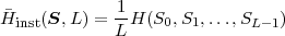 | (3.75) |
and represents the greatest lower bound for the average codeword length per symbol when a message of L symbols is coded.
Fig. 3.7 Comparison of lossless coding techniques for the stationary Markov source specified in Table 3.2 and different numbers L of coded symbols.
For L = 1 and L = 5, the scalar Huffman code and the Huffman code for blocks of 5 symbols achieve the minimum average codeword length, respectively, which confirms that Huffman codes are optimal codes for a given set of letters or letter sequences with a fixed pmf. But if more than 10 symbols are coded, all investigated Huffman codes have a lower coding efficiency than arithmetic and PIPE coding. For large numbers of coded symbols, the average codeword length for arithmetic coding approaches the entropy rate. The average codeword length for PIPE coding is only a little bit larger; the difference to arithmetic coding could be further reduced by increasing the number of probability intervals and the number of codewords for the V2V tables.
The design of Huffman codes and the coding process for arithmetic codes and PIPE codes require that the statistical properties of a source, i.e., the marginal pmf or the joint or conditional pmf’s of up to a certain order, are known. Furthermore, the local statistical properties of real data such as image and video signals usually change with time. The average codeword length can be often decreased if a lossless code is flexible and can be adapted to the local statistical properties of a source. The approaches for adaptive coding are classified into approaches with forward adaptation and approaches with backward adaptation. The basic coding structure for these methods is illustrated in Fig. 3.8.
In adaptive coding methods with forward adaptation, the statistical properties of a block of successive samples are analyzed in the encoder and an adaptation signal is included in the bitstream. This adaptation signal can be for example a Huffman code table, one or more pmf’s, or an index into a predefined list of Huffman codes or pmf’s. The decoder adjusts the used code for the block of samples according to the transmitted information. Disadvantages of this approach are that the required side information increase the transmission rate and that forward adaptation introduces a delay.
Methods with backward adaptation estimate the local statistical properties based on already coded symbols simultaneously at encoder and decoder side. As mentioned in sec. 3.2, the adaptation of Huffman codes is a quite complex task, so that backward adaptive VLC coding is rarely used in practice. But for arithmetic coding, in particular binary arithmetic coding, and PIPE coding, the backward adaptive estimation of pmf’s can be easily integrated in the coding process. Backward adaptive coding methods do not introduce a delay and do not require the transmission of any side information. However, they are not robust against transmission errors. For this reason, backward adaptation is usually only used inside a transmission packet. It is also possible to combine backward and forward adaptation. As an example, the arithmetic coding design in H.264/AVC [36] supports the transmission of a parameter inside a data packet that specifies one of three initial sets of pmf’s, which are then adapted based on the actually coded symbols.
3.8 Summary of Lossless Source Coding
We have introduced the concept of uniquely decodable codes and investigated the design of prefix codes. Prefix codes provide the useful property of instantaneous decodability and it is possible to achieve an average codeword length that is not larger than the average codeword length for any other uniquely decodable code. The measures of entropy and block entropy have been derived as lower bounds for the average codeword length for coding a single symbol and a block of symbols, respectively. A lower bound for the average codeword length per symbol for any lossless source coding technique is the entropy rate.
Huffman codes have been introduced as optimal codes that assign a separate codeword to a given set of letters or letter sequences with a fixed pmf. However, for sources with memory, an average codeword length close to the entropy rate can only be achieved if a large number of symbols is coded jointly, which requires large codeword tables and is not feasible in practical coding systems. Furthermore, the adaptation of Huffman codes to time-varying statistical properties is typically considered as too complex for video coding applications, which often have real-time requirements.
Arithmetic coding represents a fixed-precision variant of Elias coding and can be considered as a universal lossless coding method. It does not require the storage of a codeword table. The arithmetic code for a symbol sequence is iteratively constructed by successively refining a cumulative probability interval, which requires a fixed number of arithmetic operations per coded symbol. Arithmetic coding can be elegantly combined with backward adaptation to the local statistical behavior of the input source. For the coding of long symbol sequences, the average codeword length per symbol approaches the entropy rate.
As an alternative to arithmetic coding, we presented the probability interval partitioning entropy (PIPE) coding. The input symbols are binarized using simple prefix codes and the resulting sequence of binary symbols is partitioned into a small number of bin sequences, which are then coded using simple binary V2V codes. PIPE coding provides the same simple mechanism for probability modeling and backward adaptation as arithmetic coding. However, the complexity is reduced in comparison to arithmetic coding and PIPE coding provides the possibility to parallelize the encoding and decoding process. For long symbol sequences, the average codeword length per symbol is similar to that of arithmetic coding.
It should be noted that there are various other approaches to lossless coding including Lempel-Ziv coding [79], Tunstall coding [73, 66], or Burrows-Wheeler coding [7]. These methods are not considered in this text, since they are not used in the video coding area.
This is the html version of the book:
Thomas Wiegand and Heiko Schwarz (2010): "Source Coding: Part I of Fundamentals of Source and Video Coding", Now Publishers, Foundations and Trends® in Signal Processing: Vol. 4: No 1-2, pp 1-222. (pdf version of the book)
4 Rate Distortion Theory
In lossy coding, the reconstructed signal is not identical to the source signal, but represents only an approximation of it. A measure of the deviation between the approximation and the original signal is referred to as distortion. Rate distortion theory addresses the problem of determining the minimum average number of bits per sample that is required for representing a given source without exceeding a given distortion. The greatest lower bound for the average number of bits is referred to as the rate distortion function and represents a fundamental bound on the performance of lossy source coding algorithms, similarly as the entropy rate represents a fundamental bound for lossless source coding. For deriving the results of rate distortion theory, no particular coding technique is assumed. The applicability of rate distortion theory includes discrete and continuous random processes.
In this chapter, we give an introduction to rate distortion theory and derive rate distortion bounds for some important model processes. We will use these results in the following chapters for evaluating the performance of different lossy coding techniques. For further details, the reader is referred to the comprehensive treatments of the subject in [22, 4] and the overview in [11].
4.1 The Operational Rate Distortion Function
A lossy source coding system as illustrated in Fig. 4.1 consists of an encoder and a decoder. Given a sequence of source symbols s, the encoder generates a sequence of codewords b. The decoder converts the sequence of codewords b into a sequence of reconstructed symbols s′.
The encoder operation can be decomposed into an irreversible encoder mapping α, which maps a sequence of input samples s onto a sequence of indexes i, and a lossless mapping γ, which converts the sequence of indexes i into a sequence of codewords b. The encoder mapping α can represent any deterministic mapping that produces a sequence of indexes i of a countable alphabet. This includes the methods of scalar quantization, vector quantization, predictive coding, and transform coding, which will be discussed in the following chapters. The lossless mapping γ can represent any lossless source coding technique, including the techniques that we discussed in chapter 3. The decoder operation consists of a lossless mapping γ-1, which represents the inverse of the lossless mapping γ and converts the sequence of codewords b into the sequence of indexes i, and a deterministic decoder mapping β, which maps the sequence of indexes i to a sequence of reconstructed symbols s′. A lossy source coding system Q is characterized by the mappings α, β, and γ. The triple Q = (α,β,γ) is also referred to as source code or simply as code throughout this text.
A simple example for a source code is an N-dimensional block code
QN = {αN,βN,γN}, by which blocks of N consecutive input samples are
independently coded. Each block of input samples s(N) = {s0, ,sN-1} is
mapped to a vector of K quantization indexes i(K) = αN(s(N)) using a
deterministic mapping αN and the resulting vector of indexes i is converted
into a variable-length bit sequence b(ℓ) = γN(i(K)). At the decoder side, the
recovered vector i(K) = γN-1(b(ℓ)) of indexes is mapped to a block
s′(N) = βN(i(K)) of N reconstructed samples using the deterministic
decoder mapping βN.
,sN-1} is
mapped to a vector of K quantization indexes i(K) = αN(s(N)) using a
deterministic mapping αN and the resulting vector of indexes i is converted
into a variable-length bit sequence b(ℓ) = γN(i(K)). At the decoder side, the
recovered vector i(K) = γN-1(b(ℓ)) of indexes is mapped to a block
s′(N) = βN(i(K)) of N reconstructed samples using the deterministic
decoder mapping βN.
In the following, we will use the notations αN, βN, and γN also for representing the encoder, decoder, and lossless mappings for the first N samples of an input sequence, independently of whether the source code Q represents an N-dimensional block code.
For continuous random processes, the encoder mapping α cannot be invertible, since real numbers cannot be represented by indexes of a countable alphabet and they cannot be losslessly described by a finite number of bits. Consequently, the reproduced symbol sequence s′ is not the same as the original symbol sequence s. In general, if the decoder mapping β is not the inverse of the encoder mapping α, the reconstructed symbols are only an approximation of the original symbols. For measuring the goodness of such an approximation, distortion measures are defined that express the difference between a set of reconstructed samples and the corresponding original samples as a non-negative real value. A smaller distortion corresponds to a higher approximation quality. A distortion of zero specifies that the reproduced samples are identical to the corresponding original samples.
In this text, we restrict our considerations to the important class of additive distortion measures. The distortion between a single reconstructed symbol s′ and the corresponding original symbol s is defined as a function d1(s,s′), which satisfies
 | (4.1) |
with equality if and only if s = s′. Given such a distortion measure d1(s,s′), the distortion between a set of N reconstructed samples s′ = {s′0,s′1,…,s′N-1} and the corresponding original samples s = {s0,s1,…,sN-1} is defined by
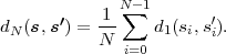 | (4.2) |
The most commonly used additive distortion measure is the squared error, d1(s,s′) = (s - s′)2. The resulting distortion measure for sets of samples is the mean squared error (MSE),
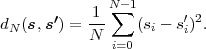 | (4.3) |
The reasons for the popularity of squared error distortion measures are their simplicity and the mathematical tractability of the associated optimization problems. Throughout this text, we will explicitly use the squared error and mean squared error as distortion measures for single samples and sets of samples, respectively. It should, however, be noted that in most video coding applications the quality of the reconstruction signal is finally judged by human observers. But the MSE does not well correlate with the quality that is perceived by human observers. Nonetheless, MSE-based quality measures are widely used in the video coding community. The investigation of alternative distortion measures for video coding applications is still an active field of research.
In order to evaluate the approximation quality of a code Q, rather than measuring distortion for a given finite symbol sequence, we are interested in a measure for the expected distortion for very long symbol sequences. Given a random process S = {Sn}, the distortion δ(Q) associated with a code Q is defined as the limit of the expected distortion as the number of coded symbols approaches infinity,
 | (4.4) |
if the limit exists. S(N) = {S0,S1,…,SN-1} represents the sequence of the first N random variables of the random process S and βN(αN(⋅)) specifies the mapping of the first N input symbols to the corresponding reconstructed symbols as given by the code Q.
For stationary processes S with a multivariate pdf f(s) and a block code QN = (αN,βN,γN), the distortion δ(QN) is given by
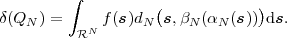 | (4.5) |
Beside the distortion δ(Q), another important property required for evaluating the performance of a code Q is its rate. For coding of a finite symbol sequence s(N), we define the transmission rate as the average number of bits per input symbol,
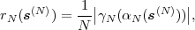 | (4.6) |
where γN(αN(⋅)) specifies the mapping of the N input symbols to the bit sequence b(ℓ) of ℓ bits as given by the code Q and the operator |⋅| is defined to return the number of bits in the bit sequence that is specified as argument. Similarly as for the distortion, we are interested in a measure for the expected number of bits per symbol for long sequences. For a given random process S = {Sn}, the rate r(Q) associated with a code Q is defined as the limit of the expected number of bits per symbol as the number of transmitted symbols approaches infinity,
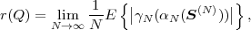 | (4.7) |
if the limit exists. For stationary random processes S and a block codes QN = (αN,βN,γN), the rate r(QN) is given by
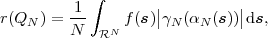 | (4.8) |
where f(s) is the N-th order joint pdf of the random process S.
4.1.3 Operational Rate Distortion Function
For a given source S, each code Q is associated with a rate distortion point (R,D), which is given by R = r(Q) and D = δ(Q). In the diagram of Fig. 4.2, the rate distortion points for selected codes are illustrated as dots. The rate distortion plane can be partitioned into a region of achievable rate distortion points and a region of non-achievable rate distortion points. A rate distortion point (R,D) is called achievable if there is a code Q with r(Q) ≤ R and δ(Q) ≤ D. The boundary between the regions of achievable and non-achievable rate distortion points specifies the minimum rate R that is required for representing the source S with a distortion less than or equal to a given value D or, alternatively, the minimum distortion D that can be achieved if the source S is coded at a rate less than or equal to a given value R. The function R(D) that describes this fundamental bound for a given source S is called the operational rate distortion function and is defined as the infimum of rates r(Q) for all codes Q that achieve a distortion δ(Q) less than or equal to D,
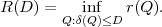 | (4.9) |
Fig. 4.2 illustrates the relationship between the region of achievable rate distortion points and the operational rate distortion function. The inverse of the operational rate distortion function is referred to as operational distortion rate function D(R) and is defined by
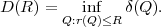 | (4.10) |
Fig. 4.2 Operational rate distortion function as boundary of the region of achievable rate distortion points. The dots represent rate distortion points for selected codes.
The terms operational rate distortion function and operational
distortion rate function are not only used for specifying the best possible
performance over all codes Q without any constraints, but also for
specifying the performance bound for sets of source codes that are
characterized by particular structural or complexity constraints. As an
example, such a set of source codes could be the class of scalar quantizers or
the class of scalar quantizers with fixed-length codewords. With  denoting
the set of source codes Q with a particular constraint, the operational rate
distortion function for a given source S and codes with the particular
constraint is defined by
denoting
the set of source codes Q with a particular constraint, the operational rate
distortion function for a given source S and codes with the particular
constraint is defined by
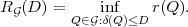 | (4.11) |
Similarly, the operational distortion rate function for a given source S and
a set of codes with a particular constraint is defined by
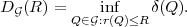 | (4.12) |
It should be noted that in contrast to information rate distortion functions, which will be introduced in the next section, operational rate distortion functions are not convex. They are more likely to be step functions, i.e., piecewise constant functions.
4.2 The Information Rate Distortion Function
In the previous section, we have shown that the operational rate distortion function specifies a fundamental performance bound for lossy source coding techniques. But unless we suitably restrict the set of considered codes, it is virtually impossible to determine the operational rate distortion function according to the definition in (4.9). A more accessible expression for a performance bound of lossy codes is given by the information rate distortion function, which was originally introduced by Shannon in [69, 70].
In the following, we first introduce the concept of mutual information before we define the information rate distortion function and investigate its relationship to the operational rate distortion function.
Although this chapter deals with the lossy coding of random sources, we will introduce the quantity of mutual information for general random variables and vectors of random variables.
Let X and Y be two discrete random variables with alphabets
X = {x0,x1, ,xMX-1} and Y = {y0,y1,
 ,yMY -1}, respectively.
As shown in sec. 3.2, the entropy H(X) represents a lower bound
for the average codeword length of a lossless source code for the
random variable X. It can also be considered as a measure for the
uncertainty that is associated with the random variable X or as a measure
for the average amount of information that is required to describe
the random variable X. The conditional entropy H(X|Y ) can be
interpreted as a measure for the uncertainty that we have about the
random variable X if we observe the random variable Y or as the
average amount of information that is required to describe the random
variable X if the random variable Y is known. The mutual information
between the discrete random variables X and Y is defined as the
difference
,yMY -1}, respectively.
As shown in sec. 3.2, the entropy H(X) represents a lower bound
for the average codeword length of a lossless source code for the
random variable X. It can also be considered as a measure for the
uncertainty that is associated with the random variable X or as a measure
for the average amount of information that is required to describe
the random variable X. The conditional entropy H(X|Y ) can be
interpreted as a measure for the uncertainty that we have about the
random variable X if we observe the random variable Y or as the
average amount of information that is required to describe the random
variable X if the random variable Y is known. The mutual information
between the discrete random variables X and Y is defined as the
difference
 | (4.13) |
The mutual information I(X;Y ) is a measure for the reduction of the uncertainty about the random variable X due to the observation of Y . It represents the average amount of information that the random variable Y contains about the random variable X. Inserting the formulas for the entropy (3.13) and conditional entropy (3.20) yields
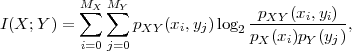 | (4.14) |
where pX and pY represent the marginal pmf’s of the random variables X and Y , respectively, and pXY denotes the joint pmf.
For extending the concept of mutual information to general random variables we consider two random variables X and Y with marginal the pdf’s fX and fY , respectively, and the joint pdf fXY . Either or both of the random variables may be discrete or continuous or of mixed type. Since the entropy, as introduced in sec. 3.2, is only defined for discrete random variables, we investigate the mutual information for discrete approximations XΔ and Y Δ of the random variables X and Y .
With Δ being a step size, the alphabet of the discrete approximation
XΔ of a random variable X is defined by XΔ = {…,x-1,x0,x1,…} with
xi = i ⋅ Δ. The event {XΔ = xi} is defined to be equal to the event
{xi ≤ X < xi+1}. Furthermore, we define an approximation fX(Δ) of the
pdf fX for the random variable X, which is constant inside each
half-open interval [xi,xi+1), as illustrated in Fig. 4.3, and is given
by
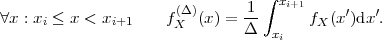 | (4.15) |
The pmf pXΔ for the random variable XΔ can then be expressed as
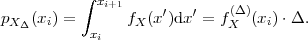 | (4.16) |
Similarly, we define a piecewise constant approximation fXY (Δ) for the joint pdf fXY of two random variables X and Y , which is constant inside each 2-dimensional interval [xi,xi+1) × [yj,yj+1). The joint pmf pXΔY Δ of the two discrete approximations XΔ and Y Δ is then given by
 | (4.17) |
Using the relationships (4.16) and (4.17), we obtain for the mutual information of the discrete random variables XΔ and Y Δ
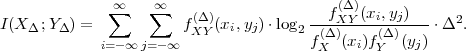 | (4.18) |
If the step size Δ approaches zero, the discrete approximations XΔ and Y Δ approach the random variables X and Y . The mutual information I(X;Y ) for random variables X and Y can be defined as limit of the mutual information I(XΔ;Y Δ) as Δ approaches zero,
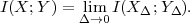 | (4.19) |
If the step size Δ approaches zero, the piecewise constant pdf approximations fXY (Δ), fX(Δ), and fY (Δ) approach the pdf’s fXY , fX, and fY , respectively, and the sum in (4.18) approaches the integral
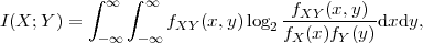 | (4.20) |
which represents the definition of mutual information.
The formula (4.20) shows that the mutual information I(X;Y ) is
symmetric with respect to the random variables X and Y . The average
amount of information that a random variable X contains about another
random variable Y is equal to the average amount of information
that Y contains about X. Furthermore, the mutual information
I(X;Y ) is greater than or equal to zero, with equality if and only if
fXY (x,y) = fX(x)fY (x), ∀x,y ∈ , i.e., if and only if the random
variables X and Y are independent. This is a direct consequence of
the divergence inequality for probability density functions f and
g,
, i.e., if and only if the random
variables X and Y are independent. This is a direct consequence of
the divergence inequality for probability density functions f and
g,
 | (4.21) |
which is fulfilled with equality if and only if the pdfs f and g are the same. The divergence inequality can be proved using the inequality lnx ≥ x - 1 (with equality if and only if x = 1),
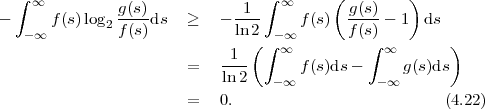
For N-dimensional random vectors X = (X0,X1,…,XN-1)T and Y = (Y 0,Y 1,…,Y N-1)T , the definition of mutual information can be extended according to
 | (4.23) |
where fX and fY denote the marginal pdfs for the random vectors X and Y , respectively, and fXY represents the joint pdf.
We now assume that the random vector Y is a discrete random vector
and is associated with an alphabet Y N. Then, the pdf fY and the
conditional pdf fY |X can be written as
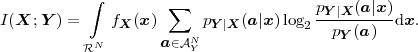 | (4.26) |
This expression can be re-written as
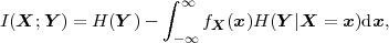 | (4.27) |
where H(Y ) is the entropy of the discrete random vector Y and
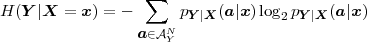 | (4.28) |
is the conditional entropy of Y given the event {X = x}. Since the conditional entropy H(Y |X = x) is always nonnegative, we have
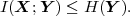 | (4.29) |
Equality is obtained if and only if H(Y |X = x) is zero for all x and, hence, if and only if the random vector Y is given by a deterministic function of the random vector X.
If we consider two random processes X = {Xn} and Y = {Y n} and represent the random variables for N consecutive time instants as random vectors X(N) and Y (N), the mutual information I(X(N);Y (N)) between the random vectors X(N) and Y (N) is also referred to as N-th order mutual information and denoted by IN(X;Y ).
4.2.2 Information Rate Distortion Function
Suppose we have a source S = {Sn} that is coded using a lossy source coding system given by a code Q = (α,β,γ). The output of the lossy coding system can be described by the random process S′ = {S′n}. Since coding is a deterministic process given by the mapping β(α(⋅)), the random process S′ describing the reconstructed samples is a deterministic function of the input process S. Nonetheless, the statistical properties of the deterministic mapping given by a code Q can be described by a conditional pdf gQ(s′|s) = gS′n|Sn(s′|s). If we consider, as an example, simple scalar quantization, the conditional pdf gQ(s′|s) represents, for each value of s, a shifted Dirac delta function. In general, gQ(s′|s) consists of a sum of scaled and shifted Dirac delta functions. Note that the random variables S′n are always discrete and, hence, the conditional pdf gQ(s′|s) can also be represented by a conditional pmf. Instead of single samples, we can also consider the mapping of blocks of N successive input samples S to blocks of N successive output samples S′. For each value of N > 0, the statistical properties of a code Q can then be described by the conditional pdf gNQ(s′|s) = gS′|S(s′|s).
For the following considerations, we define the N-th order distortion
 | (4.30) |
Given a source S, with an N-th order pdf fS, and an additive distortion measure dN, the N-th order distortion δN(gN) is completely determined by the conditional pdf gN = gS′|S. The distortion δ(Q) that is associated with a code Q and was defined in (4.4) can be written as
 | (4.31) |
Similarly, the N-th order mutual information IN(S;S′) between blocks of N successive input samples and the corresponding blocks of output samples can be written as
 | (4.32) |
with
 | (4.33) |
For a given source S, the N-th order mutual information only depends on the N-th order conditional pdf gN.
We now consider any source code Q with a distortion δ(Q) that is less than or equal to a given value D. As mentioned above, the output process S′ of a source coding system is always discrete. We have shown in sec. 3.3.1 that the average codeword length for lossless coding of a discrete source cannot be smaller than the entropy rate of the source. Hence, the rate r(Q) of the code Q is greater than or equal to the entropy rate of S′,
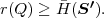 | (4.34) |
By using the definition of the entropy rate (S′) in (3.25) and the relationship (4.29), we obtain
 | (4.35) |
where HN(S′) denotes the block entropy for the random vectors S′ of N successive reconstructed samples and IN(S;S′) is the mutual information between the N-dimensional random vectors S and the corresponding reconstructions S′. A deterministic mapping as given by a source code is a special case of a random mapping. Hence, the N-th order mutual information IN(gNQ) for a particular code Q with δN(gNQ) ≤ D cannot be smaller than the smallest N-th order mutual information IN(gN) that can be achieved using any random mapping gN = gS′|S with δN(gN) ≤ D,
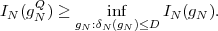 | (4.36) |
Consequently, the rate r(Q) is always greater than or equal to
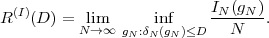 | (4.37) |
This fundamental lower bound for all lossy source coding techniques is called the information rate distortion function. Every code Q that yields a distortion δ(Q) less than or equal to any given value D for a source S is associated with a rate r(Q) that is greater than or equal to the information rate distortion function R(I)(D) for the source S,
 | (4.38) |
This relationship is called the fundamental source coding theorem. The information rate distortion function was first derived by Shannon for iid sources [69, 70] and is for that reason also referred to as Shannon rate distortion function.
If we restrict our considerations to iid sources, the N-th order joint pdf
fS(s) can be represented as the product ∏
i=0N-1fS(si) of the marginal
pdf fS(s), with s = {s0, ,sN-1}. Hence, for every N, the N-th order
distortion δN(gNQ) and mutual information IN(gNQ) for a code Q can be
expressed using a scalar conditional pdf gQ = gS′|S,
,sN-1}. Hence, for every N, the N-th order
distortion δN(gNQ) and mutual information IN(gNQ) for a code Q can be
expressed using a scalar conditional pdf gQ = gS′|S,
 | (4.39) |
Consequently, the information rate distortion function R(I)(D) for iid sources is equal to the so-called first order information rate distortion function,
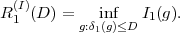 | (4.40) |
In general, the function
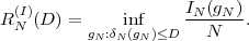 | (4.41) |
is referred to as the N-th order information rate distortion function. If N approaches infinity, the N-th order information rate distortion function approaches the information rate distortion function,
 | (4.42) |
We have shown that the information rate distortion function represents a fundamental lower bound for all lossy coding algorithms. Using the concept of typical sequences, it can additionally be shown that the information rate distortion function is also asymptotically achievable [4, 22, 11], meaning that for any ε > 0 there exists a code Q with δ(Q) ≤ D and r(Q) ≤ R(I)(D) + ε. Hence, subject to suitable technical assumptions the information rate distortion function is equal to the operational rate distortion function. In the following text, we use the notation R(D) and the term rate distortion function to denote both the operational and information rate distortion function. The term operational rate distortion function will mainly be used for denoting the operational rate distortion function for restricted classes of codes.
The inverse of the information rate distortion function is called the information distortion rate function or simply the distortion rate function and is given by
 | (4.43) |
Using this definition, the fundamental source coding theorem (4.38) can also be written as
 | (4.44) |
The information rate distortion function is defined as a mathematical function of a source. However, an analytical derivation of the information rate distortion function is still very difficult or even impossible, except for some special random processes. An iterative technique for numerically computing close approximations of the rate distortion function for iid sources was developed by Blahut and Arimoto in [6, 3] and is referred to as Blahut-Arimoto algorithm. An overview of the algorithm can be found in [22, 11].
4.2.3 Properties of the Rate Distortion Function
In the following, we state some important properties of the rate distortion function R(D) for the MSE distortion measure11 The properties hold more generally. In particular, all stated properties are valid for additive distortion measures for which the single-letter distortion d1(s,s′) is equal to zero if s = s′ and is greater than zero if s≠s′. . For proofs of these properties, the reader is referred to [4, 22, 11].
 | (4.45) |
For the MSE distortion measure, the value of Dmax is equal to the variance σ2 of the source.
 | (4.46) |
The last property shows that the fundamental bound for lossless coding is a special case of the fundamental bound for lossy coding.
For most random processes, an analytical expression for the rate distortion function cannot be given. In the following, we show how a useful lower bound for the rate distortion function of continuous random processes can be calculated. Before we derive this so-called Shannon lower bound, we introduce the quantity of differential entropy.
The mutual information I(X;Y ) of two continuous N-dimensional random vectors X and Y is defined in (4.23). Using the relationship fXY = fX|Y ⋅ fY , the integral in this definition can be decomposed into a part that only depends on one of the random vectors and a part that depends on both random vectors,
 | (4.47) |
with
and In analogy to the discrete entropy introduced in Chapter 3, the quantity h(X) is called the differential entropy of the random vector X and the quantity h(X|Y ) is referred to as conditional differential entropy of the random vector X given the random vector Y .Since I(X;Y ) is always nonnegative, we can conclude that conditioning reduces the differential entropy,
 | (4.50) |
similarly as conditioning reduces the discrete entropy.
For continuous random processes S = {Sn}, the random variables Sn
for N consecutive time instants can be represented as a random vector
S(N) = (S0, ,SN-1)T . The differential entropy h(S(N)) for the
vectors S(N) is then also referred to as N-th order differential entropy and
is denoted by
,SN-1)T . The differential entropy h(S(N)) for the
vectors S(N) is then also referred to as N-th order differential entropy and
is denoted by
 | (4.51) |
If, for a continuous random process S, the limit
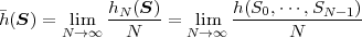 | (4.52) |
exists, it is called the differential entropy rate of the process S.
The differential entropy has a different meaning than the discrete entropy. This can be illustrated by considering an iid process S = {Sn} with a uniform pdf f(s), with f(s) = 1∕A for |s|≤ A∕2 and f(s) = 0 for |s| > A∕2. The first order differential entropy for this process is
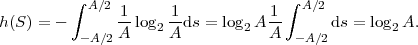 | (4.53) |
In Fig. 4.4, the differential entropy h(S) for the uniform iid process is shown as function of the parameter A. In contrast to the discrete entropy, the differential entropy can be either positive or negative. The discrete entropy is only finite for discrete alphabet sources, it is infinite for continuous alphabet sources. The differential entropy, however, is mainly useful for continuous random processes. For discrete random processes, it can be considered to be minus infinity.
As an example, we consider a stationary Gaussian random process with a mean μ and an N-th order autocovariance matrix CN. The N-th order pdf fG(s) is given in (2.51), where μN represents a vector with all N elements being equal to the mean μ. For the N-th order differential entropy hN(G) of the stationary Gaussian process, we obtain
By reformulating the matrix multiplication in the last integral as sum, it can be shown that for any random process with an N-th order pdf f(s) and an N-th order autocovariance matrix CN,
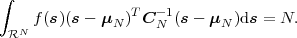 | (4.55) |
A step-by-step derivation of this result can be found in [11]. Inserting (4.55) into (4.54) and using log 2e = (ln2)-1 yields
Now, we consider any stationary random process S with a mean μ and an N-th order autocovariance matrix CN. The N-th order pdf of this process is denoted by f(s). Using the divergence inequality (4.21), we obtain for its N-th order differential entropy,
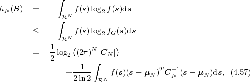
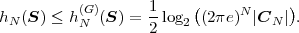 | (4.58) |
Hence, the N-th order differential entropy of any stationary non-Gaussian process is less than the N-th order differential entropy of a stationary Gaussian process with the same N-th order autocovariance matrix CN.
As shown in (4.56), the N-th order differential entropy of a stationary Gaussian process depends on the determinant of its N-th order autocovariance matrix |CN|. The determinant |CN| is given by the product of the eigenvalues ξi of the matrix CN, |CN| = ∏ i=0N-1ξi. The trace of the N-th order autocovariance matrix tr(CN) is given by the sum of its eigenvalues, tr(CN) = ∑ i=0N-1ξi, and, according to (2.39), also by tr(CN) = N ⋅ σ2, with σ2 being the variance of the Gaussian process. Hence, for a given variance σ2, the sum of the eigenvalues is constant. With the inequality of arithmetic and geometric means,
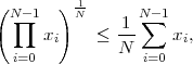 | (4.59) |
which holds with equality if and only if x0 = x1 = … = xN-1, we obtain the inequality
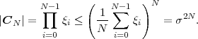 | (4.60) |
Equality holds if and only if all eigenvalues of CN are the same, i.e, if and only if the Gaussian process is iid. Consequently, the N-th order differential entropy of a stationary process S with a variance σ2 is bounded by
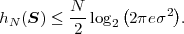 | (4.61) |
It is maximized if and only if the process is a Gaussian iid process.
Using the relationship (4.47) and the notation IN(gN) = IN(S;S′), the rate distortion function R(D) defined in (4.37) can be written as
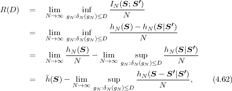
Since conditioning reduces the differential entropy, as has been shown in (4.50), the rate distortion function is bounded by
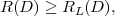 | (4.63) |
with
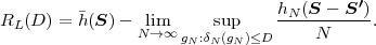 | (4.64) |
The lower bound RL(D) is called the Shannon lower bound (SLB).
For stationary processes and the MSE distortion measure, the distortion
δN(gN) in (4.64) is equal to the variance σZ2 of the process Z = S -S′.
Furthermore, we have shown in (4.61) that the maximum N-th order
differential entropy for a stationary process with a given variance σZ2 is
equal to  log 2(2πeσZ2). Hence, the Shannon lower bound for stationary
processes and MSE distortion is given by
log 2(2πeσZ2). Hence, the Shannon lower bound for stationary
processes and MSE distortion is given by
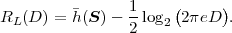 | (4.65) |
Since we concentrate on the MSE distortion measure in this text, we call RL(D) given in (4.65) the Shannon lower bound in the following without mentioning that it is only valid for the MSE distortion measure.
The N-th order differential entropy for iid sources S = {Sn} is equal to
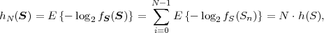 | (4.66) |
where h(S) denotes the first order differential entropy. Hence, the Shannon lower bound for iid sources is given by
In the following, the differential entropy h(S) and the Shannon lower bound DL(R) are given for three distributions. For the example of the Laplacian iid process with σ2 = 1, Fig. 4.5 compares the Shannon lower bound DL(R) with the distortion rate function D(R), which was calculated using the Blahut-Arimoto algorithm [6, 3].
Uniform pdf:
 | (4.69) |
Laplacian pdf:
 | (4.70) |
Gaussian pdf:
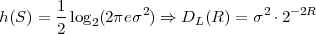 | (4.71) |
Fig. 4.5 Comparison of the Shannon lower bound DL(R) and the distortion rate function D(R) for a Laplacian iid source with unit variance (σ2 = 1).
The comparison of the Shannon lower bound DL(R) and the distortion rate function D(R) for the Laplacian iid source in Fig. 4.5 indicates that the Shannon lower bound approaches the distortion rate function for small distortions or high rates. For various distortion measures, including the MSE distortion, it can in fact be shown that the Shannon lower bound approaches the rate distortion function as the distortion approaches zero,
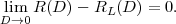 | (4.72) |
Consequently, the Shannon lower bound represents a suitable reference for the evaluation of lossy coding techniques at high rates or small distortions. Proofs for the asymptotic tightness of the Shannon lower bound for various distortion measures can be found in [48, 5, 47].
For sources with memory, an exact analytic derivation of the Shannon lower bound is usually not possible. One of the few examples for which the Shannon lower bound can be expressed analytically is the stationary Gaussian process. The N-th order differential entropy for a stationary Gaussian process has been derived in (4.56). Inserting this result into the definition of the Shannon lower bound (4.65) yields
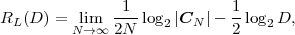 | (4.73) |
where CN is the N-th order autocorrelation matrix. The determinant of a matrix is given by the product of its eigenvalues. With ξi(N), for i = 0,1,…,N - 1, denoting the N eigenvalues of the N-th order autocorrelation matrix CN, we obtain
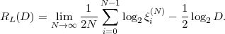 | (4.74) |
In order to proceed, we restrict our considerations to Gaussian processes with zero mean, in which case the autocovariance matrix CN is equal to the autocorrelation matrix RN, and apply Grenander and Szegö’s theorem [29] for sequences of Toeplitz matrices. For a review of Toeplitz matrices, including the theorem for sequences of Toeplitz matrices, we recommend the tutorial [23]. Grenander and Szegö’s theorem can be stated as follows: If RN is a sequence of Hermitian Toeplitz matrices with elements ϕk on the k-th diagonal, the infimum Φinf = inf ωΦ(ω) and supremum Φsup = supωΦ(ω) of the Fourier series
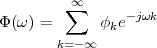 | (4.75) |
are finite, and the function G is continuous in the interval [Φinf,Φsup], then
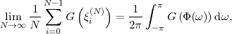 | (4.76) |
where ξi(N), for i = 0,1,…,N - 1, denote the eigenvalues of the N-th matrix RN.
A matrix is called Hermitian if it is equal to its conjugate transpose. This property is always fulfilled for real symmetric matrices as the autocorrelation matrices of stationary processes. Furthermore, the Fourier series (4.75) for the elements of the autocorrelation matrix RN is the power spectral density ΦSS(ω). If we assume that the power spectral density is finite and greater than 0 for all frequencies ω, the limit in (4.74) can be replaced by an integral according to (4.76). The Shannon lower bound RL(D) of a stationary Gaussian process with zero-mean and a power spectral density ΦSS(ω) is given by
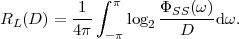 | (4.77) |
A nonzero mean does not have any impact on the Shannon lower bound RL(D), but on the power spectral density ΦSS(ω).
For a stationary zero-mean Gauss-Markov process, the entries of the autocorrelation matrix are given by ϕk = σ2ρ|k|, where σ2 is the signal variance and ρ is the correlation coefficient between successive samples. Using the relationship ∑ k=1∞ake-jkx = a∕(e-jx - a), we obtain
Inserting this relationship into (4.77) yields where we used ∫ 0π ln(a2 - 2abcosx + b2)dx = 2π lna, for a ≥ b > 0. As discussed above, the mean of a stationary process does not have any impact on the Shannon rate distortion function or the Shannon lower bound. Hence, the distortion rate function DL(R) for the Shannon lower bound of a stationary Gauss-Markov process with a variance σ2 and a correlation coefficient ρ is given by
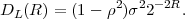 | (4.80) |
This result can also be obtained by directly inserting the formula (2.50) for the determinant |CN| of the N-th order autocovariance matrix for Gauss-Markov processes into the expression (4.73).
4.4 Rate Distortion Function for Gaussian Sources
Stationary Gaussian sources play a fundamental role in rate distortion theory. We have shown that the Gaussian source maximize the differential entropy, and thus also the Shannon lower bound, for a given variance or autocovariance function. Stationary Gaussian sources are also one of the few examples, for which the rate distortion function can be exactly derived.
Before stating another important property of Gaussian iid sources, we calculate their rate distortion function. Therefore, we first derive a lower bound and then show that this lower bound is achievable. To prove that the lower bound is achievable, it is sufficient to show that there is a conditional pdf gS′|S(s′|s) for which the mutual information I1(gS′|S) is equal to the lower bound for a given distortion D.
The Shannon lower bound for Gaussian iid sources as distortion rate function DL(R) has been derived in sec. 4.3. The corresponding rate distortion function is given by
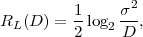 | (4.81) |
where σ2 is the signal variance. For proving that the rate distortion function is achievable, it is more convenient to look at the pdf of the reconstruction fS′(s′) and the conditional pdf gS|S′(s|s′) of the input given the reconstruction.
For distortions D < σ2, we choose
where μ denotes the mean of the Gaussian iid process. It should be noted that the conditional pdf gS|S′ represents a Gaussian pdf for the random variables Zn = Sn - S′n, which are given by the difference of the corresponding random variables Sn and S′n. We now verify that the pdf fS(s) that we obtain with the choices (4.82) and (4.83) represents the Gaussian pdf with a mean μ and a variance σ2. Since the random variables Sn can be represented as the sum S′n + Zn, the pdf fS(s) is given by the convolution of fS′(s′) and gS|S′(s|s′). And since means and variances add when normal densities are convolved, the pdf fS(s) that is obtained is a Gaussian pdf with a mean μ = μ + 0 and a variance σ2 = (σ2 - D) + D. Hence, the choices (4.82) and (4.83) are valid, and the conditional pdf gS′|S(s′|s) could be calculated using Bayes rule
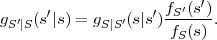 | (4.84) |
The resulting distortion is given by the variance of the difference process Zn = Sn - S′n,
 | (4.85) |
For the mutual information, we obtain
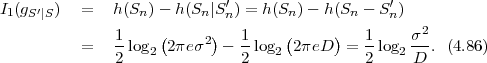
The results show that, for any distortion D < σ2, we can find a conditional pdf gS′|S that achieves the Shannon lower bound. For greater distortions, we choose gS′|S(s′|s) = δ(0), which gives a distortion of σ2 and a rate of zero. Consequently, the rate distortion function for Gaussian iid sources is given by
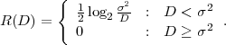 | (4.87) |
The corresponding distortion rate function is given by
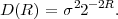 | (4.88) |
It is important to note that the rate distortion function for a Gaussian iid process is equal to the Shannon lower bound for the entire range of rates. Furthermore, it can be shown [4] that for every iid process with a given variance σ2, the rate distortion function lies below that of the Gaussian iid process with the same variance.
4.4.2 Gaussian Sources with Memory
For deriving the rate distortion function R(D) for a stationary Gaussian process with memory, we decompose it into a number N of independent stationary Gaussian sources. The N-th order rate distortion function RN(D) can then be expressed using the rate distortion function for Gaussian iid processes and the rate distortion function R(D) is obtained by considering the limit of RN(D) as N approaches infinity.
As we stated in sec. 2.3, the N-th order pdf of a stationary Gaussian process is given by
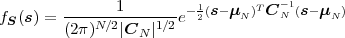 | (4.89) |
where s is a vector of N consecutive samples, μN is a vector with all N elements being equal to the mean μ, and CN is the N-th order autocovariance matrix. Since CN is a symmetric and real matrix, it has N real eigenvalues ξi(N), for i = 0,1,…,N - 1. The eigenvalues are solutions of the equation
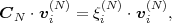 | (4.90) |
where vi(N) represents a nonzero vector with unit norm, which is called a unit-norm eigenvector corresponding to the eigenvalue ξi(N). Let AN be the matrix whose columns are build by the N unit-norm eigenvectors,
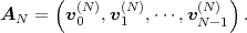 | (4.91) |
By combining the N equations (4.90) for i = 0,1,…,N - 1, we obtain the matrix equation
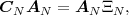 | (4.92) |
where
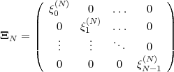 | (4.93) |
is a diagonal matrix that contains the N eigenvalues of CN on its main diagonal. The eigenvectors are orthogonal to each other and AN is an orthogonal matrix.
Given the stationary Gaussian source {Sn}, we construct a source {Un} by decomposing the source {Sn} into vectors S of N successive random variables and applying the transform
 | (4.94) |
to each of these vectors. Since AN is orthogonal, its inverse A-1 exists and is equal to its transpose AT . The resulting source {Un} is given by the concatenation of the random vectors U. Similarly, the inverse transform for the reconstructions {U′n} and {S′n} is given by
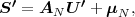 | (4.95) |
with U′ and S′ denoting the corresponding vectors of N successive random variables. Since the coordinate mapping (4.95) is the inverse of the mapping (4.94), the N-th order mutual information IN(U;U′) is equal to the N-th order mutual information IN(S;S′). A proof of this statement can be found in [4]. Furthermore, since AN is orthogonal, the transform
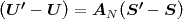 | (4.96) |
preserves the Euclidean norm22 We will show in sec. 7.2 that every orthogonal transform preserves the MSE distortion. . The MSE distortion between any realization s of the random vector S and its reconstruction s′
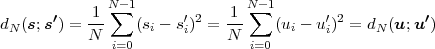 | (4.97) |
is equal to the distortion between the corresponding vector u and its reconstruction u′. Hence, the N-th order rate distortion function RN(D) for the stationary Gaussian source {Sn} is equal to the N-th order rate distortion function for the random process {Un}.
A linear transformation of a Gaussian random vector results in another Gaussian random vector. For the mean vector and the autocorrelation matrix of U, we obtain
 | (4.98) |
and
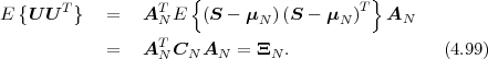
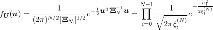 | (4.100) |
of the pdf’s of the Gaussian components Ui. Consequently, the components Ui are independent of each other.
In sec. 4.2.2, we have shown how the N-th order mutual information and the N-th order distortion for a code Q can be described by a conditional pdf gNQ = gU′|U that characterizes the mapping of the random vectors U onto the corresponding reconstruction vectors U′. Due to the independence of the components Ui of the random vectors U, the N-th order mutual information IN(gNQ) and the N-th order distortion δN(gNQ) for a code Q can be written as
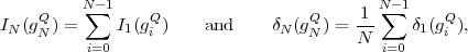 | (4.101) |
where giQ = gU′i|Ui specifies the conditional pdf for the mapping of a vector component Ui onto its reconstruction U′i. Consequently, the N-th order distortion rate function DN(R) can be expressed by
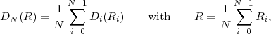 | (4.102) |
where Ri(Di) denotes the first order rate distortion function for a vector component Ui. The first order distortion rate function for Gaussian sources has been derived in sec. 4.4.1 and is given by
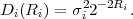 | (4.103) |
The variances σi2 of the vector component Ui are equal to the eigenvalues ξi(N) of the N-th order autocovariance matrix CN. Hence, the N-th order distortion rate function can be written as
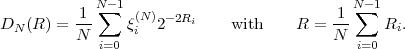 | (4.104) |
With the inequality of arithmetic and geometric means, which holds with equality if and only if all elements have the same value, we obtain
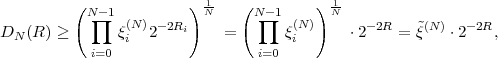 | (4.105) |
where  (N) denotes the geometric mean of the eigenvalues ξi(N). For a given
N-th order mutual information R, the distortion is minimized if and only
if ξi(N)2-2Ri is equal to
(N) denotes the geometric mean of the eigenvalues ξi(N). For a given
N-th order mutual information R, the distortion is minimized if and only
if ξi(N)2-2Ri is equal to  (N)2-2R for all i = 0,
 ,N - 1, which
yields
,N - 1, which
yields
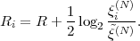 | (4.106) |
In the above result, we have ignored the fact that the mutual
information Ri for a component Ui cannot be less than zero. Since the
distortion rate function given in (4.103) is steeper at low Ri, the mutual
information Ri for components with ξi(N) <  (N)2-2R has to be set equal
to zero and the mutual information R has to be distributed among the
remaining components in order to minimize the distortion. This can be
elegantly specified by introducing a parameter θ, with θ ≥ 0, and setting
the component distortions according to
(N)2-2R has to be set equal
to zero and the mutual information R has to be distributed among the
remaining components in order to minimize the distortion. This can be
elegantly specified by introducing a parameter θ, with θ ≥ 0, and setting
the component distortions according to
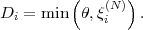 | (4.107) |
This concept is also know as inverse water-filling for independent Gaussian sources [57], where the parameter θ can be interpreted as the water level. Using (4.103), we obtain for the mutual information Ri,
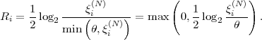 | (4.108) |
The N-th order rate distortion function RN(D) can be expressed by the following parametric formulation, with θ ≥ 0,
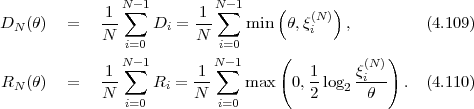
The rate distortion function R(D) for the stationary Gaussian random process {Sn} is given by the limit
 | (4.111) |
which yields the parametric formulation, with θ > 0,
 | (4.112) |
For Gaussian processes with zero mean (CN = RN), we can apply the theorem for sequences of Toeplitz matrices (4.76) to express the rate distortion function using the power spectral density ΦSS(ω) of the source. A parametric formulation, with θ ≥ 0, for the rate distortion function R(D) for a stationary Gaussian source with zero mean and a power spectral density ΦSS(ω) is given by
The minimization in the parametric formulation (4.113) and (4.114) of
the rate distortion function is illustrated in Fig. 4.6. It can be interpreted
that at each frequency, the variance of the corresponding frequency
component as given by the power spectral density ΦSS(ω) is compared to
the parameter θ, which represents the mean squared error of the frequency
component. If ΦSS(ω) is found to be larger than θ, the mutual information
is set equal to  log 2
log 2 , otherwise a mutual information of zero is
assigned to that frequency component.
, otherwise a mutual information of zero is
assigned to that frequency component.
Fig. 4.6 Illustration of parametric equations for the rate distortion function of stationary Gaussian processes.
For stationary zero-mean Gauss-Markov sources with a variance σ2 and a correlation coefficient ρ, the power spectral density ΦSS(ω) is given by (4.78). If we choose the parameter θ according to
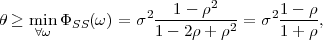 | (4.115) |
we obtain the parametric equations
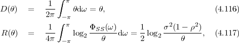
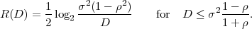 | (4.118) |
Conversely, for rates R ≥ log 2(1 + ρ), the distortion rate function of a stationary Gauss-Markov process coincides with Shannon lower bound,
 | (4.119) |
For Gaussian iid sources (ρ = 0), these results are identical to (4.87) and (4.88). Fig. 4.7 shows distortion rate functions for stationary Gauss-Markov processes with different correlation factors ρ. The distortion is plotted as signal-to-noise ratio SNR = 10log 10(σ2∕D).
Fig. 4.7 Distortion rate functions for Gauss-Markov processes with different correlation factors ρ. The distortion D is plotted as signal-to-noise ratio SNR = 10 log 10(σ2∕D).
We have noted above that the rate distortion function of the Gaussian iid process with a given variance specifies an upper bound for the rate distortion functions of all iid processes with the same variance. This statement can be generalized to stationary Gaussian processes with memory. The rate distortion function of the stationary zero-mean Gaussian process as given parametrically by (4.113) and (4.114) specifies an upper limit for the rate distortion functions of all other stationary processes with the same power spectral density ΦSS(ω). A proof of this statement can be found in [4].
4.5 Summary of Rate Distortion Theory
Rate distortion theory addresses the problem of finding the greatest lower bound for the average number of bits that is required for representing a signal without exceeding a given distortion. We introduced the operational rate distortion function that specifies this fundamental bound as infimum of over all source codes. A fundamental result of rate distortion theory is that the operational rate distortion function is equal to the information rate distortion function, which is defined as infimum over all conditional pdf’s for the reconstructed samples given the original samples. Due to this equality, both the operational and the information rate distortion function are usually referred to as the rate distortion function. It has further been noted that, for the MSE distortion measure, the lossless coding theorem specifying that the average codeword length per symbol cannot be less than the entropy rate represents a special case of rate distortion theory for discrete sources with zero distortion.
For most sources and distortion measures, it is not known how to analytically derive the rate distortion function. A useful lower bound for the rate distortion function is given by the so-called Shannon lower bound. The difference between the Shannon lower bound and the rate distortion function approaches zero as the distortion approaches zero or the rate approaches infinity. Due to this property, it represents a suitable reference for evaluating the performance of lossy coding schemes at high rates. For the MSE distortion measure, an analytical expression for the Shannon lower bound can be given for typical iid sources as well as for general stationary Gaussian sources.
An important class of processes is the class of stationary Gaussian processes. For Gaussian iid processes and MSE distortion, the rate distortion function coincides with the Shannon lower bound for all rates. The rate distortion function for general stationary Gaussian sources with zero mean and MSE distortion can be specified as a parametric expression using the power spectral density. It has also been noted that the rate distortion function of the stationary Gaussian process with zero mean and a particular power spectral density represents an upper bound for all stationary processes with the same power spectral density, which leads to the conclusion that Gaussian sources are the most difficult to code.
This is the html version of the book:
Thomas Wiegand and Heiko Schwarz (2010): "Source Coding: Part I of Fundamentals of Source and Video Coding", Now Publishers, Foundations and Trends® in Signal Processing: Vol. 4: No 1-2, pp 1-222. (pdf version of the book)
5 Quantization
Lossy source coding systems, which we have introduced in chapter 4, are characterized by the fact that the reconstructed signal is not identical to the source signal. The process that introduces the corresponding loss of information (or signal fidelity) is called quantization. An apparatus or algorithmic specification that performs the quantization process is referred to as quantizer. Each lossy source coding system includes a quantizer. The rate distortion point associated with a lossy source coding system is to a wide extent determined by the used quantization process. For this reason, the analysis of quantization techniques is of fundamental interest for the design of source coding systems.
In this chapter, we analyze the quantizer design and the performance of various quantization techniques with the emphasis on scalar quantization, since it is the most widely used quantization technique in video coding. To illustrated the inherent limitation of scalar quantization, we will also briefly introduce the concept of vector quantization and show its advantage with respect to the achievable rate distortion performance. For further details, the reader is referred to the comprehensive treatment of quantization in [16] and the overview of the history and theory of quantization in [28].
5.1 Structure and Performance of Quantizers
In the broadest sense, quantization is an irreversible deterministic mapping of an input quantity to an output quantity. For all cases of practical interest, the set of obtainable values for the output quantity is finite and includes fewer elements than the set of possible values for the input quantity. If the input quantity and the output quantity are scalars, the process of quantization is referred to as scalar quantization. A very simple variant of scalar quantization is the rounding of a real input value to its nearest integer value. Scalar quantization is by far the most popular form of quantization and is used in virtually all video coding applications. However, as we will see later, there is a gap between the operational rate distortion curve for optimal scalar quantizers and the fundamental rate distortion bound. This gap can only be reduced if a vector of more than one input sample is mapped to a corresponding vector of output samples. In this case, the input and output quantity are vectors and the quantization process is referred to as vector quantization. Vector quantization can asymptotically achieve the fundamental rate distortion bound if the number of samples in the input and output vector approaches infinity.
A quantizer Q of dimension N specifies a mapping
of the N-dimensional Euclidean space N into a
finite
set of reconstruction vectors inside the N-dimensional Euclidean space
N,
(Although we restrict our considerations to finite sets of reconstruction vectors, some of the
presented quantization methods and derivations are also valid for countably infinite sets of
reconstruction vectors.)
 | (5.1) |
If the dimension N of the quantizer Q is equal to 1, it is a scalar quantizer;
otherwise, it is a vector quantizer. The number K of reconstruction vectors
is also referred to as the size of the quantizer Q. The deterministic
mapping Q associates a subset i of the N-dimensional Euclidean
space N with each of the reconstruction vectors s′i. The subsets
i, with 0 ≤ i < K, are called quantization cells and are defined
by
 | (5.2) |
From this definition, it follows that the quantization cells i form a
partition of the N-dimensional Euclidean space N,
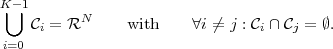 | (5.3) |
Given the quantization cells i and the associated reconstruction
values s′i, the quantization mapping Q can be specified by
 | (5.4) |
A quantizer is completely specified by the set of reconstruction values and the associated quantization cells.
For analyzing the design and performance of quantizers, we consider the
quantization of symbol sequences {sn} that represent realizations of a
random process {Sn}. For the case of vector quantization (N > 1), the
samples of the input sequence {sn} shall be arranged in vectors, resulting
in a sequence of symbol vectors {sn}. Usually, the input sequence {sn} is
decomposed into blocks of N samples and the components of an input
vector sn are build be the samples of such a block, but other arrangements
are also possible. In any case, the sequence of input vectors {sn} can be
considered to represent a realization of a vector random process {Sn}. It
should be noted that the domain of the input vectors sn can be a subset of
the N-dimensional space N, which is the case if the random process {Sn}
is discrete or its marginal pdf f(s) is zero outside a finite interval. However,
even in this case, we can generally consider quantization as a mapping of
the N-dimensional Euclidean space N into a finite set of reconstruction
vectors.
Fig. 5.1 shows a block diagram of a quantizer Q. Each input vector sn is mapped onto one of the reconstruction vectors, given by Q(sn). The average distortion D per sample between the input and output vectors depends only on the statistical properties of the input sequence {sn} and the quantization mapping Q. If the random process {Sn} is stationary, it can be expressed by
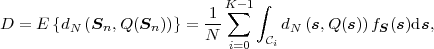 | (5.5) |
where fS denotes the joint pdf of the vector components of the random vectors Sn. For the MSE distortion measure, we obtain
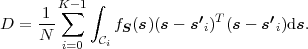 | (5.6) |
Unlike the distortion D, the average transmission rate is not only determined by the quantizer Q and the input process. As illustrated in Fig. 5.1, we have to consider the lossless coding γ by which the sequence of reconstruction vectors {Q(sn)} is mapped onto a sequence of codewords. For calculating the performance of a quantizer or for designing a quantizer we have to make reasonable assumptions about the lossless coding γ. It is certainly not a good idea to assume a lossless coding with an average codeword length per symbol close to the entropy for the design, but to use the quantizer in combination with fixed-length codewords for the reconstruction vectors. Similarly, a quantizer that has been optimized under the assumption of fixed-length codewords is not optimal if it is used in combination with advanced lossless coding techniques such as Huffman coding or arithmetic coding.
The rate R of a coding system consisting of a quantizer Q and a lossless coding γ is defined as the average codeword length per input sample. For stationary input processes {Sn}, it can be expressed by
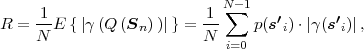 | (5.7) |
where |γ(s′i)| denotes the average codeword length that is obtained for a reconstruction vector s′i with the lossless coding γ and p(s′i) denotes the pmf for the reconstruction vectors, which is given by
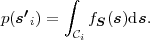 | (5.8) |
The probability of a reconstruction vector does not depend on the
reconstruction vector itself, but only on the associated quantization
cell i.
Fig. 5.2 Lossy source coding system consisting of a quantizer, which is decomposed into an encoder mapping α and a decoder mapping β, and a lossless coder γ.
A quantizer Q can be decomposed into two parts, an encoder mapping α which maps the input vectors sn to quantization indexes i, with 0 ≤ i < K, and a decoder mapping β which maps the quantization indexes i to the associated reconstruction vectors s′i. The quantizer mapping can then be expressed by Q(s) = α(β(s)). The loss of signal fidelity is introduced as a result of the encoder mapping α, the decoder mapping β merely maps the quantization indexes i to the associated reconstruction vectors s′i. The combination of the encoder mapping α and the lossless coding γ forms an encoder of a lossy source coding system as illustrated in Fig. 5.2. The corresponding decoder is given by the inverse lossless coding γ-1 and the decoder mapping β.
In scalar quantization (N = 1), the input and output quantity are
scalars. Hence, a scalar quantizer Q of size K specifies a mapping of the
real line into a set of K reconstruction levels,
 | (5.9) |
In the general case, a quantization cell i corresponds to a set of intervals
of the real line. We restrict our considerations to regular scalar quantizers
for which each quantization cell i represents a single interval of the real
line and the reconstruction levels s′i are located inside the associated
quantization cells i. Without loss of generality, we further assume
that the quantization cells are ordered in increasing order of the
values of their lower interval boundary. When we further assume
that the quantization intervals include the lower, but not the higher
interval boundary, each quantization cell can be represented by a
half-open22 In strict mathematical sense, the first quantization cell is an open interval  0 = (-∞,u1).
interval i = [ui,ui+1). The interval boundaries ui are also referred to
as decision thresholds. The interval sizes Δi = ui+1 - ui are called
quantization step sizes. Since the quantization cells must form a
partition of the real line , the values u0 and uK are fixed and
given by u0 = -∞ and uK = ∞. Consequently, K reconstruction
levels and K -1 decision thresholds can be chosen in the quantizer
design.
0 = (-∞,u1).
interval i = [ui,ui+1). The interval boundaries ui are also referred to
as decision thresholds. The interval sizes Δi = ui+1 - ui are called
quantization step sizes. Since the quantization cells must form a
partition of the real line , the values u0 and uK are fixed and
given by u0 = -∞ and uK = ∞. Consequently, K reconstruction
levels and K -1 decision thresholds can be chosen in the quantizer
design.
The quantizer mapping Q of a scalar quantizer as defined above can be represented by a piecewise-constant input-output function as illustrated in Fig. 5.3. All input values s with ui ≤ s < ui+1 are assigned to the corresponding reproduction level s′i.
In the following treatment of scalar quantization, we generally assume that the input process is stationary. For continuous random processes, scalar quantization can then can be interpreted as a discretization of the marginal pdf f(s) as illustrated in Fig. 5.4.
For any stationary process {S} with a marginal pdf f(s), the quantizer output is a discrete random process {S′} with a marginal pmf
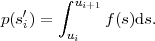 | (5.10) |
The average distortion D (for the MSE distortion measure) is given by
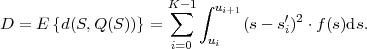 | (5.11) |
The average rate R depends on the lossless coding γ and is given by
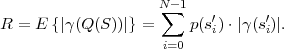 | (5.12) |
5.2.1 Scalar Quantization with Fixed-Length Codes
We will first investigate scalar quantizers in connection with fixed-length codes. The lossless coding γ is assumed to assign a codeword of the same length to each reconstruction level. For a quantizer of size K, the codeword length must be greater than or equal to ⌈log 2K⌉. Under these assumptions, the quantizer size K should be a power of 2. If K is not a power of 2, the quantizer requires the same minimum codeword length as a quantizer of size K′ = 2⌈log 2K⌉, but since K < K′, the quantizer of size K′ can achieve a smaller distortion. For simplifying the following discussion, we define the rate R according to
 | (5.13) |
but inherently assume that K represents a power of 2.
A very simple form of quantization is the pulse-code-modulation (PCM) for random processes with a finite amplitude range. PCM is a quantization process for which all quantization intervals have the same size Δ and the reproduction values s′i are placed in the middle between the decision thresholds ui and ui+1. For general input signals, this is not possible since it results in an infinite number of quantization intervals K and hence an infinite rate for our fixed-length code assumption. However, if the input random process has a finite amplitude range of [smin,smax], the quantization process is actually a mapping of the finite interval [smin,smax] to the set of reproduction levels. Hence, we can set u0 = smin and uK = smax. The width A = smax - smin of the amplitude interval is then evenly split into K quantization intervals, resulting in a quantization step size
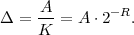 | (5.14) |
The quantization mapping for PCM can be specified by
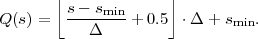 | (5.15) |
As an example, we consider PCM quantization of a stationary random
process with an uniform distribution, f(s) =  for -
for - ≤ s ≤
≤ s ≤ . The
distortion as defined in (5.11) becomes
. The
distortion as defined in (5.11) becomes
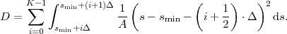 | (5.16) |
By carrying out the integration and inserting (5.14), we obtain the operational distortion rate function,
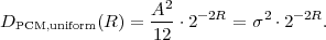 | (5.17) |
For stationary random processes with an infinite amplitude range, we have to choose u0 = -∞ and uK = ∞. The inner interval boundaries ui, with 0 < i < K, and the reconstruction levels s′i can be evenly distributed around the mean value μ of the random variables S. For symmetric distributions (μ = 0), this gives
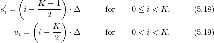
Fig. 5.5 PCM quantization of stationary random processes with uniform (U), Laplacian (L), and Gaussian (G) distributions: (left) operational distortion rate functions in comparison to the corresponding Shannon lower bounds (for variances σ2 = 1); (right) optimal quantization step sizes.
For the application of PCM quantization to stationary random processes with an infinite amplitude interval, we have chosen the quantization step size for a given quantizer size K by minimizing the distortion. A natural extension of this concept is to minimize the distortion with respect to all parameters of a scalar quantizer of a given size K. The optimization variables are the K - 1 decision thresholds ui, with 0 < i < K, and the K reconstruction levels s′i, with 0 ≤ i < K. The obtained quantizer is called a pdf-optimized scalar quantizer with fixed-length codes.
For deriving a condition for the reconstruction levels s′i, we first assume
that the decision thresholds ui are given. The overall distortion (5.11) is
the sum of the distortions Di for the quantization intervals i = [ui,uu+1).
For given decision thresholds, the interval distortions Di are mutually
independent and are determined by the corresponding reconstruction
levels s′i,
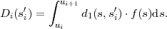 | (5.20) |
By using the conditional distribution f(s|s′i) = f(s) ⋅ p(s′i), we obtain
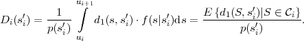 | (5.21) |
Since p(s′i) does not depend on s′i, the optimal reconstruction levels s′i* are given by
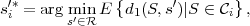 | (5.22) |
which is also called the generalized centroid condition. For the squared error distortion measure d1(s,s′) = (s - s′)2, the optimal reconstruction levels s′i* are the conditional means (centroids)
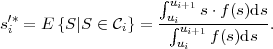 | (5.23) |
This can be easily proved by the inequality
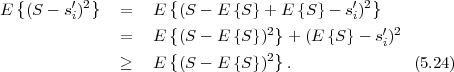
If the reproduction levels s′i are given, the overall distortion D is minimized if each input value s is mapped to the reproduction level s′i that minimizes the corresponding sample distortion d1(s,s′i),
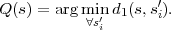 | (5.25) |
This condition is also referred to as the nearest neighbor condition. Since a decision threshold ui influences only the distortions Di of the neighboring intervals, the overall distortion is minimized if
 | (5.26) |
holds for all decision thresholds ui, with 0 < i < K. For the squared error distortion measure, the optimal decision thresholds ui*, with 0 < i < K, are given by
 | (5.27) |
The expressions (5.23) and (5.27) can also be obtained by setting the partial derivatives of the distortion (5.11) with respect to the decision thresholds ui and the reconstruction levels s′i equal to zero [56].
The necessary conditions for the optimal reconstruction levels (5.22) and decision thresholds (5.25) depend on each other. A corresponding iterative algorithm for minimizing the distortion of a quantizer of given size K was suggested by Lloyd [49] and is commonly called the Lloyd algorithm. The obtained quantizer is referred to as Lloyd quantizer or Lloyd-Max33 Lloyd and Max independently observed the two necessary conditions for optimality. quantizer. For a given pdf f(s), first an initial set of unique reconstruction levels {s′i} is arbitrarily chosen, then the decision thresholds {ui} and reconstruction levels {s′i} are alternately determined according to (5.25) and (5.22), respectively, until the algorithm converges. It should be noted that the fulfillment of the conditions (5.22) and (5.25) is in general not sufficient to guarantee the optimality of the quantizer. The conditions are only sufficient if the pdf f(s) is log-concave. One of the examples, for which the Lloyd algorithm yields a unique solution independent of the initial set of reconstruction levels, is the Gaussian pdf.
Often, the marginal pdf f(s) of a random process is not known a priori. In such a case, the Lloyd algorithm can be applied using a training set. If the training set includes a sufficiently large number of samples, the obtained quantizer is an accurate approximation of the Lloyd quantizer. Using the encoder mapping α (see sec. 5.1), the Lloyd algorithm for a training set of samples {sn} and a given quantizer size K can be stated as follows:
i according to

and update the decision thresholds {ui} accordingly.

where the expectation value is taken over the training set.
As a first example, we applied the Lloyd algorithm with a training set of more than 10000 samples and the MSE distortion measure to a Gaussian pdf with unit variance. We used two different initializations for the reconstruction levels. Convergence was determined if the relative distortion reduction between two iterations steps was less than 1%, (Dk - Dk+1)∕Dk+1 < 0.01. The algorithm quickly converged after 6 iterations for both initializations to the same overall distortion DF *. The obtained reconstruction levels {s′i} and decision thresholds {ui} as well as the iteration processes for the two initializations are illustrated in Fig. 5.6.
Fig. 5.6 Lloyd algorithm for a Gaussian pdf with unit variance and two initializations: (top) final reconstruction levels and decision thresholds; (middle) reconstruction levels and decision thresholds as function of the iteration step; (bottom) overall SNR and SNR for the quantization intervals as function of the iteration step.
The same algorithm with the same two initializations was also applied to a Laplacian pdf with unit variance. Also for this distribution, the algorithm quickly converged after 6 iterations for both initializations to the same overall distortion DF *. The obtained quantizer and the iteration processes are illustrated in Fig. 5.7.
Fig. 5.7 Lloyd algorithm for a Laplacian pdf with unit variance and two initializations: (top) final reconstruction levels and decision thresholds; (middle) reconstruction levels and decision thresholds as function of the iteration step; (bottom) overall SNR and SNR for the quantization intervals as function of the iteration step.
5.2.2 Scalar Quantization with Variable-Length Codes
We have investigated the design of quantizers that minimize the distortion for a given number K of reconstruction levels, which is equivalent to a quantizer optimization using the assumption that all reconstruction levels are signaled with codewords of the same length. Now we consider the quantizer design in combination with variable-length codes γ.
The average codeword length that is associated with a particular reconstruction level s′i is denoted by (s′i) = |γ(s′i)|. If we use a scalar Huffman code, (s′i) is equal to the length of the codeword that is assigned to s′i. According to (5.12), the average rate R is given by
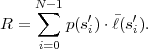 | (5.28) |
The average distortion is the same as for scalar quantization with fixed-length codes and is given by (5.11).
Since distortion and rate influence each other, they cannot be minimized independently. The optimization problem can be stated as
 | (5.29) |
or equivalently,
 | (5.30) |
with Rmax and Dmax being a given maximum rate and a maximum distortion, respectively. The constraint minimization problem can be formulated as unconstrained minimization of the Lagrangian functional
 | (5.31) |
The parameter λ, with 0 ≤ λ < ∞, is referred to as Lagrange parameter. The solution of the minimization of (5.31) is a solution of the constrained minimization problems (5.29) and (5.30) in the following sense: If there is a Lagrangian parameter λ that yields a particular rate Rmax (or particular distortion Dmax), the corresponding distortion D (or rate R) is a solution of the constraint optimization problem.
In order to derive necessary conditions similarly as for the quantizer design with fixed-length codes, we first assume that the decision thresholds ui are given. Since the rate R is independent of the reconstruction levels s′i, the optimal reconstruction levels are found by minimizing the distortion D. This is the same optimization problem as for the scalar quantizer with fixed-length codes. Hence, the optimal reconstruction levels s′i* are given by the generalized centroid condition (5.22).
The optimal average codeword lengths (s′i) also depend only on the decision thresholds ui. Given the decision thresholds and thus the probabilities p(s′i), the average codeword lengths (s′i) can be determined. If we, for example, assume that the reconstruction levels are coded using a scalar Huffman code, the Huffman code could be constructed given the pmf p(s′i), which directly yields the codeword length (s′i). In general, it is however justified to approximate the average rate R by the entropy H(S) and set the average codeword length equal to
 | (5.32) |
This underestimates the true rate by a small amount. For Huffman coding the difference is always less than 1 bit per symbol and for arithmetic coding it is usually much smaller. When using the entropy as approximation for the rate during the quantizer design, the obtained quantizer is also called an entropy-constrained scalar quantizer. At this point, we ignore that, for sources with memory, the lossless coding γ can employ dependencies between output samples, for example, by using block Huffman coding or arithmetic coding with conditional probabilities. This extension is discussed in sec. 5.2.6.
For deriving a necessary condition for the decision thresholds ui, we now assume that the reconstruction levels s′i and the average codeword length (s′i) are given. Similarly as for the nearest neighbor condition in sec. 5.2.1, the quantization mapping Q(s) that minimizes the Lagrangian functional J is given by
 | (5.33) |
A mapping Q(s) that that minimizes the term d(s,s′i) + λ(s′i) for each source symbol s minimizes also the expected value in (5.31). A rigorous proof of this statement can be found in [71]. The decision thresholds ui have to be selected in a way that the term d(s,s′i) + λ(s′i) is the same for both neighboring intervals,
 | (5.34) |
For the MSE distortion measure, we obtain
 | (5.35) |
The consequence is a shift of the decision threshold ui from the midpoint between the reconstruction levels toward the interval with the longer average codeword length, i.e., the less probable interval.
Fig. 5.8 Lagrangian minimization: (left) independent operational distortion rate curves for the 5 symbols, where each circle represents one of 6 available distortion rate points; (right) the small dots show the average distortion and rate for all possible combinations of the 5 different quantizers with their 6 rate distortion points, the circles show the solutions to the Lagrangian minimization problem.
Lagrangian minimization as in (5.33) is a very important concept in modern video coding. Hence, we have conducted a simple experiment to illustrate the minimization approach. For that, we simulated the encoding of a 5-symbol sequence {si}. The symbols are assumed to be mutually independent and have different distributions. We have generated one operational distortion rate function Di(R) = ai22-2R for each symbol, with ai2 being randomly chosen. For each operational distortion rate function we have selected 6 rate points Ri,k, which represent the available quantizers.
The Lagrangian optimization process is illustrated in Fig. 5.8. The diagram on the left shows the 5 operational distortion rate functions Di(R) with the available rate points Ri,k. The right diagram shows the average distortion and rate for each combination of rate points for encoding the 5-symbol sequence. The results of the minimization of Di(Ri,k) + λRi,k with respect to Ri,k for different values of the Lagrange parameter λ are marked by circles. This experiment illustrates that the Lagrangian minimization approach yields a result on the convex hull of the admissible distortion rate points.
Given the necessary conditions for an optimal quantizer with variable-length codes, we can construct an iterative design algorithm similar to the Lloyd algorithm. If we use the entropy as measure for the average rate, the algorithm is also referred to as entropy-constrained Lloyd algorithm. Using the encoder mapping α, the variant that uses a sufficiently large training set {sn} can be stated as follows for a given value of λ:
i according to
and update the decision thresholds {ui} accordingly.

where the expectation value is taken over the training set.
As mentioned above, the entropy constraint in the algorithm causes a shift of the cost function depending on the pmf p(s′i). If two decoding symbols s′i and s′i+1 are competing, the symbol with larger popularity has higher chance of being chosen. The probability of a reconstruction level that is rarely chosen is further reduced. As a consequence, symbols get “removed” and the quantizer size K of the final result can be smaller than the initial quantizer size N.
The number N of initial reconstruction levels is critical to quantizer performance after convergence. Fig. 5.9 illustrates the result of the entropy-constrained Lloyd algorithm after convergence for a Laplacian pdf and different numbers of initial reconstruction levels, where the rate is measured as the entropy of the reconstruction symbols. It can be seen that a larger number of initial reconstruction levels always leads to a smaller or equal distortion (higher or equal SNR) at the same rate than a smaller number of initial reconstruction levels.
Fig. 5.9 Operational distortion rate curves after convergence of the entropy-constrained Lloyd algorithm for different numbers of initialized reconstruction levels. The rate R is measured as the entropy of the reconstruction symbols.
As a first example, we applied the entropy-constrained Lloyd algorithm with the MSE distortion to a Gaussian pdf with unit variance. The resulting average distortion DF * is 10.45 dB for an average rate R, measured as entropy, of 2 bit per symbol. The obtained optimal reconstruction levels and decision thresholds are depicted in Fig. 5.10. This figure also illustrates the iteration process for two different initializations. For initialization A, the initial number of reconstruction levels is sufficiently large and during the iteration process the size of the quantizer is reduced. With initialization B, however, the desired quantizer performance is not achieved, because the number of initial reconstruction levels is too small for the chosen value of λ.
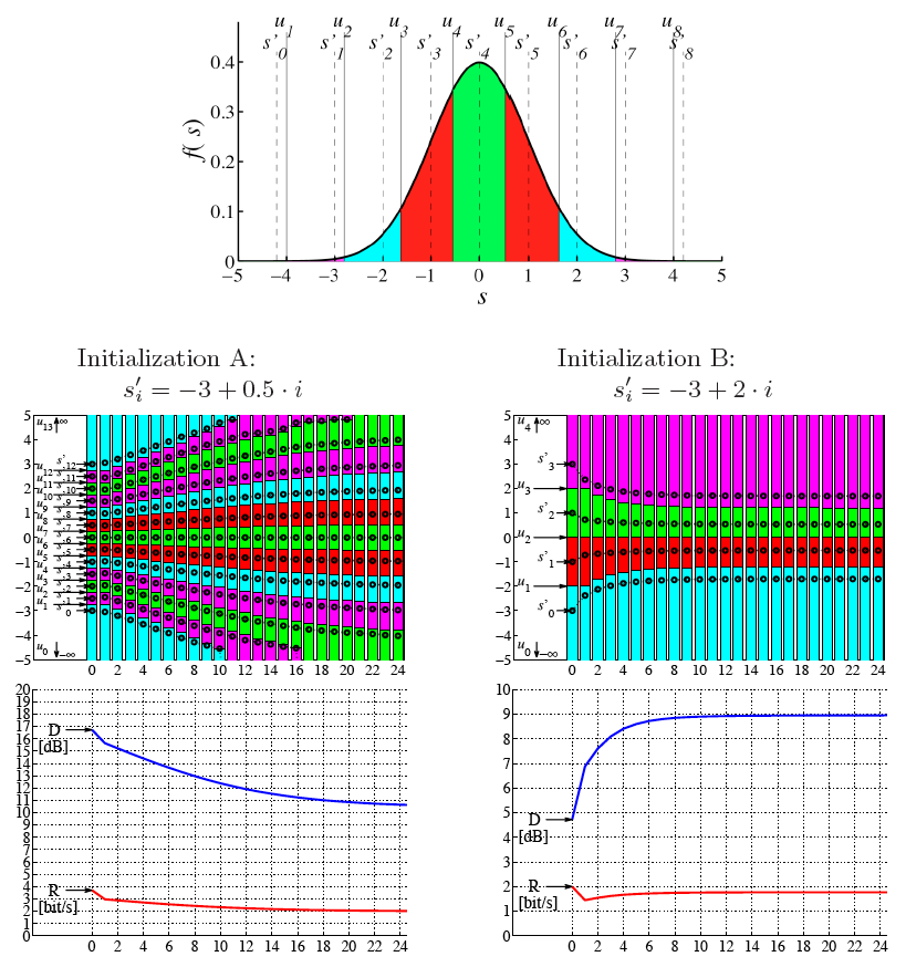 Fig. 5.10 Entropy-constrained Lloyd algorithm for a Gaussian pdf with unit variance
and two initializations: (top) final reconstruction levels and decision thresholds; (middle)
reconstruction levels and decision thresholds as function of the iteration step; (bottom)
overall distortion D and rate R, measured as entropy, as function of the iteration step.
Fig. 5.10 Entropy-constrained Lloyd algorithm for a Gaussian pdf with unit variance
and two initializations: (top) final reconstruction levels and decision thresholds; (middle)
reconstruction levels and decision thresholds as function of the iteration step; (bottom)
overall distortion D and rate R, measured as entropy, as function of the iteration step.
The same experiment was done for a Laplacian pdf with unit variance. Here, the resulting average distortion DF * is 11.46 dB for an average rate R, measured as entropy, of 2 bit per symbol. The obtained optimal reconstruction levels and decision thresholds as well as the iteration processes are illustrated in Fig. 5.11. Similarly as for the Gaussian pdf, the number of initial reconstruction levels for the initialization B is too small for the chosen value of λ, so that the desired quantization performance is not achieved. For initialization A, the initial quantizer size is large enough and the number of quantization intervals is reduced during the iteration process.
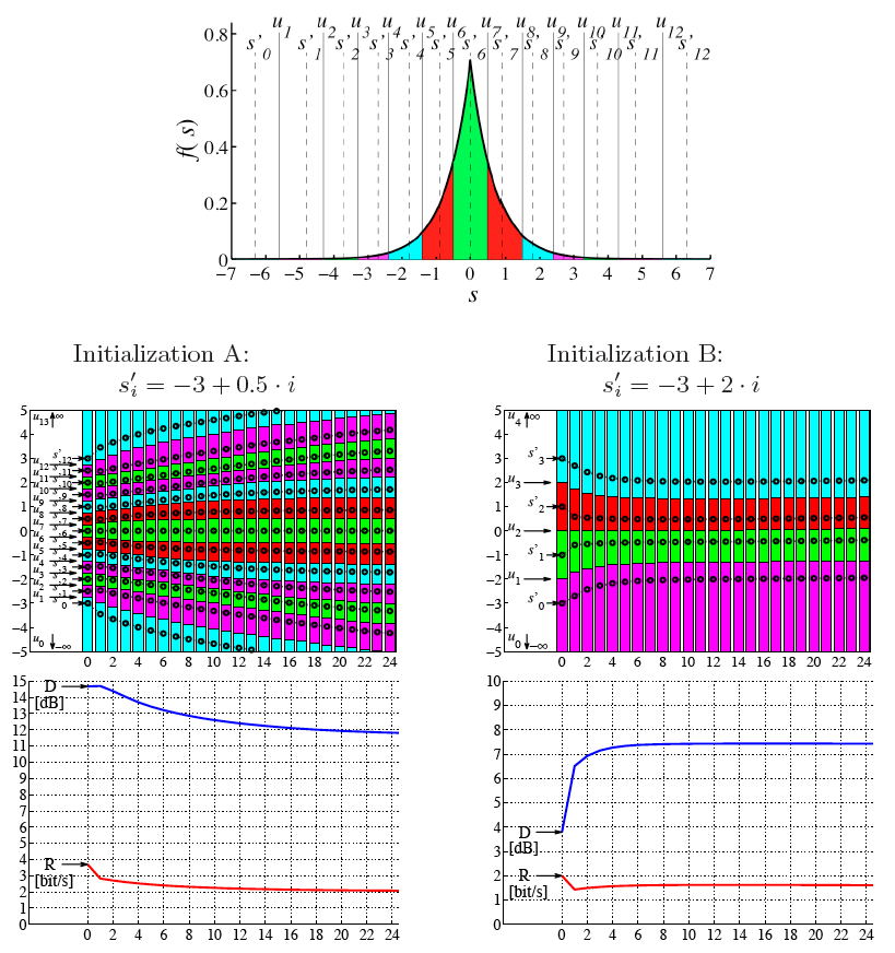 Fig. 5.11 Entropy-constrained Lloyd algorithm for a Laplacian pdf with unit variance
and two initializations: (top) final reconstruction levels and decision thresholds; (middle)
reconstruction levels and decision thresholds as function of the iteration step; (bottom)
overall distortion D and rate R, measured as entropy, as function of the iteration step.
Fig. 5.11 Entropy-constrained Lloyd algorithm for a Laplacian pdf with unit variance
and two initializations: (top) final reconstruction levels and decision thresholds; (middle)
reconstruction levels and decision thresholds as function of the iteration step; (bottom)
overall distortion D and rate R, measured as entropy, as function of the iteration step.
5.2.3 High-Rate Operational Distortion Rate Functions
In general, it is impossible to analytically state the operational distortion rate function for optimized quantizer designs. One of the few exceptions is the uniform distribution, for which the operational distortion rate function for all discussed quantizer designs is given in (5.17). For stationary input processes with continuous random variables, we can, however, derive the asymptotic operational distortion rate functions for very high rates (R →∞) or equivalently for small distortions (D → 0). The resulting relationships are referred to as high-rate approximations and approach the true operational distortion rate functions as the rate approaches infinity. We remember that as the rate approaches infinity, the (information) distortion rate function approaches the Shannon lower bound. Hence, for high rates, the performance of a quantizer design can be evaluated by comparing the high rate approximation of the operational distortion rate function with the Shannon lower bound.
The general assumption that we use for deriving high-rate approximations is that the sizes Δi of the quantization intervals [ui,ui+1) are so small that the marginal pdf f(s) of a continuous input process is nearly constant inside each interval,
 | (5.36) |
The probabilities of the reconstruction levels can be approximated by
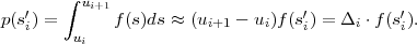 | (5.37) |
For the average distortion D, we obtain
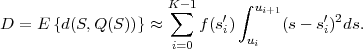 | (5.38) |
An integration of the right side of (5.38) yields
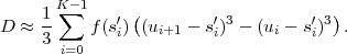 | (5.39) |
For each quantization interval, the distortion is minimized if the term (ui+1 - s′i)3 is equal to the term (ui - s′i)3, which yields
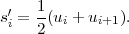 | (5.40) |
By inserting (5.40) into (5.39), we obtain the following expression for the average distortion at high rates,
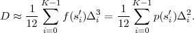 | (5.41) |
For deriving the asymptotic operational distortion rate functions, we will use the expression (5.41) with equality, but keep in mind that it is only asymptotically correct for Δi → 0.
For PCM quantization of random processes with a finite amplitude range of width A, we can directly insert the expression (5.14) into the distortion approximation (5.41). Since ∑ i=0K-1p(s′i) is equal to 1, this yields the asymptotic operational distortion rate function
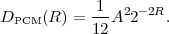 | (5.42) |
In order to derive the asymptotic operational distortion rate function for optimal scalar quantizers in combination with fixed-length codes, we again start with the distortion approximation in (5.41). By using the relationship ∑ i=0K-1K-1 = 1, it can be reformulated as
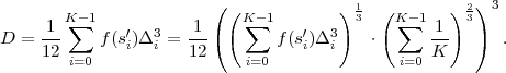 | (5.43) |
Using Hölders inequality
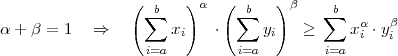 | (5.44) |
with equality if and only if xi is proportional to yi, it follows
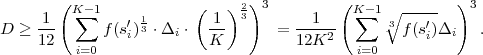 | (5.45) |
Equality is achieved if the terms f(s′i)Δi3 are proportional to 1∕K. Hence, the average distortion for high rates is minimized if all quantization intervals have the same contribution to the overall distortion D.
We have intentionally chosen α = 1∕3, in order to obtain an expression of the sum in which Δi has no exponent. Remembering that the used distortion approximation is asymptotically valid for small intervals Δi, the summation in (5.45) can be written as integral,
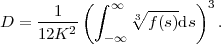 | (5.46) |
As discussed in sec. 5.2.1, the rate R for a scalar quantizer with fixed-length codes is given by R = log 2K. This yields the following asymptotic operational distortion rate function for optimal scalar quantizers with fixed-length codes,
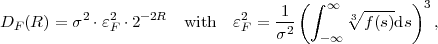 | (5.47) |
where the factor εF 2 only depends on the marginal pdf f(s) of the input process. The result (5.47) was reported by Panter and Dite in [59] and is also referred to as the Panter and Dite formula.
In sec. 5.2.2, we have discussed that the rate R for an optimized scalar quantizer with variable-length codes can be approximated by the entropy H(S′) of the output random variables S′. We ignore that, for the quantization of sources with memory, the output samples are not mutually independent and hence a lossless code that employs the dependencies between the output samples may achieve a rate below the scalar entropy H(S′).
By using the entropy H(S′) of the output random variables S′ as approximation for the rate R and applying the high-rate approximation p(s′i) = f(s′i)Δi, we obtain
Since we investigate the asymptotic behavior for small interval sizes Δi, the first term in (5.48) can be formulated as an integral, which actually represents the differential entropy h(S), yielding We continue with applying Jensen’s inequality for convex functions φ(x), such as φ(x) = -log 2x, and positive weights ai,
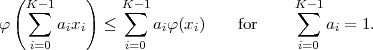 | (5.50) |
By additionally using the distortion approximation (5.41), we obtain
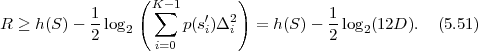
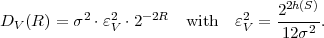 | (5.52) |
Similarly as for the Panter and Dite formula, the factor εF 2 only depends on the marginal pdf f(s) of the input process. This result (5.52) was established by Gish and Pierce in [17] using variational calculus and is also referred to as Gish and Pierce formula. The use of Jensen’s inequality to obtain the same result was first published in [27].
We now compare the asymptotic operational distortion rate functions for the discussed quantizer designs with the Shannon lower bound (SLB) for iid sources. All high-rate approximations and also the Shannon lower bound can be written as
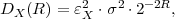 | (5.53) |
where the subscript X stands for optimal scalar quantizers with fixed-length codes (F), optimal scalar quantizers with variable-length codes (V ), or the Shannon lower bound (L). The factors εX2 depend only on the pdf f(s) of the source random variables. For the high-rate approximations, εF 2 and εV 2 are given by (5.47) and (5.52), respectively. For the Shannon lower bound, εL2 is equal to 22h(S)∕(2πe) as can be easily derived from (4.68). Table 5.1 provides an overview of the various factors εX2 for three example distributions.
| Shannon Lower | Panter & Dite | Gish & Pierce | |
| Bound (SLB) | (Pdf-Opt w. FLC) | (Uniform Q. w. VLC) | |
| Uniform pdf |  ≈ 0.7 ≈ 0.7 | 1 | 1 |
| (1.53 dB to SLB) | (1.53 dB to SLB) | ||
| Laplacian pdf |  ≈ 0.86 ≈ 0.86 |  = 4.5 = 4.5 |  ≈ 1.23 ≈ 1.23 |
| (7.1 dB to SLB) | (1.53 dB to SLB) | ||
| Gaussian pdf | 1 |  ≈ 2.72 ≈ 2.72 |  ≈ 1.42 ≈ 1.42 |
| (4.34 dB to SLB) | (1.53 dB to SLB) | ||
If we reformulate (5.53) as signal-to-noise ratio (SNR), we obtain
 | (5.54) |
For all high-rate approximations including the Shannon lower bound, the SNR is a linear function of the rate with a slope of 20log 102 ≈ 6. Hence, for high rates the MSE distortion decreases by approximately 6 dB per bit, independently of the source distribution.
A further remarkable fact is obtained by comparing the asymptotic
operational distortion rate function for optimal scalar quantizers for
variable-length codes with the Shannon lower bound. The ratio DV (R)∕DL(R)
is constant and equal to πe∕6 ≈ 1.53 dB. The corresponding rate difference
RV (D) - RL(D) is equal to  log 2(πe∕6) ≈ 0.25. At high rates, the
distortion of an optimal scalar quantizer with variable-length codes is
only 1.53 dB larger than the Shannon lower bound. And for low
distortions, the rate increase with respect to the Shannon lower bounds
is only 0.25 bit per sample. Due to this fact, scalar quantization
with variable-length coding is extensively used in modern video
coding.
log 2(πe∕6) ≈ 0.25. At high rates, the
distortion of an optimal scalar quantizer with variable-length codes is
only 1.53 dB larger than the Shannon lower bound. And for low
distortions, the rate increase with respect to the Shannon lower bounds
is only 0.25 bit per sample. Due to this fact, scalar quantization
with variable-length coding is extensively used in modern video
coding.
5.2.4 Approximation for Distortion Rate Functions
The asymptotic operational distortion rate functions for scalar quantizers that we have derived in sec. 5.2.3 can only be used as approximations for high rates. For several optimization problems, it is however desirable to have a simple and reasonably accurate approximation of the distortion rate function for the entire range of rates. In the following, we attempt to derive such an approximation for the important case of entropy-constrained scalar quantization (ECSQ).
If we assume that the optimal entropy-constrained scalar quantizer for a particular normalized distribution (zero mean and unit variance) and its operational distortion rate function g(R) are known, the optimal quantizer for the same distribution but with different mean and variance can be constructed by an appropriate shifting and scaling of the quantization intervals and reconstruction levels. The distortion rate function D(R) of the resulting scalar quantizer can then be written as
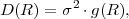 | (5.55) |
where σ2 denotes the variance of the input distribution. Hence, it is sufficient to derive an approximation for the normalized operational distortion rate function g(R).
For optimal ECSQ, the function g(R) and its derivative g′(R) should have the following properties:
 | (5.56) |
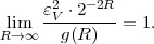 | (5.57) |
 | (5.58) |
Afunction that satisfies the above conditions is
 | (5.59) |
The factor a is chosen in a way that g(0) is equal to 1. By numerical optimization, we obtained a = 0.9519 for the Gaussian pdf and a = 0.5 for the Laplacian pdf. For proving that condition (5.57) is fulfilled, we can substitute x = 2-2R and develop the Taylor series of the resulting function
 | (5.60) |
around x0 = 0, which gives
 | (5.61) |
Since the remaining terms of the Taylor series are negligible for small values of x (large rates R), (5.59) approaches the high-rate approximation εV 22-2R as the rate R approaches infinity. The first derivative of (5.59) is given by
 | (5.62) |
It is a continuous and always less than zero.
Fig. 5.12 Operational distortion rate functions for a Gaussian (left) and Laplacian (right) pdf with unit variance. The diagrams show the (information) distortion rate function, the high-rate approximation εV 22-2R, and the approximation g(R) given in (5.59). Additionally, results of the EC-Lloyd algorithm with the rate being measured as entropy are shown.
The quality of the approximations for the operational distortion rate functions of an entropy-constrained quantizer for a Gaussian and Laplacian pdf is illustrated in Fig. 5.12. For the Gaussian pdf, the approximation (5.59) provides a sufficiently accurate match to the results of the entropy-constrained Lloyd algorithm and will be used later. For the Laplacian pdf, the approximation is less accurate for low bit rates.
5.2.5 Performance Comparison for Gaussian Sources
In the following, we compare the rate distortion performance of the discussed scalar quantizers designs with the rate distortion bound for unit-variance stationary Gauss-Markov sources with ρ = 0 and ρ = 0.9. The distortion rate functions for both sources, the operational distortion rates function for PCM (uniform, fixed-rate), the Lloyd design, and the entropy-constraint Lloyd design (EC-Lloyd), as well as the Panter & Dite and Gish & Pierce asymptotes are depicted in Fig. 5.13. The rate for quantizers with fixed-length codes is given by the binary logarithm of the quantizer size K. For quantizers with variable-length codes, it is measured as the entropy of the reconstruction levels.
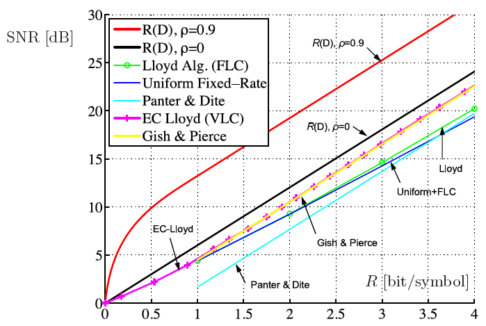
The scalar quantizer designs behave identical for both sources as only the marginal pdf f(s) is relevant for the quantizer design algorithms. For high rates, the entropy-constrained Lloyd design and the Gish & Pierce approximation yield an SNR that is 1.53 dB smaller than the (information) distortion rate function for the Gauss-Markov source with ρ = 0. The rate distortion performance of the quantizers with fixed-length codes is worse, particularly for rates above 1 bit per sample. It is, however, important to note that it cannot be concluded that the Lloyd algorithm yields a worse performance than the entropy-constrained Lloyd algorithm. Both quantizers are (locally) optimal with respect to their application area. The Lloyd algorithm results an optimized quantizer for fixed-length coding, while the entropy-constrained Lloyd algorithm yields on optimized quantizer for variable-length coding (with an average codeword length close to the entropy).
The distortion rate function for the Gauss-Markov source with ρ = 0.9 is far away from the operational distortion rate functions of the investigated scalar quantizer designs. The reason is that we assumed a lossless coding γ that achieves a rate close to the entropy H(S′) of the output process. A combination of scalar quantization and advanced lossless coding techniques that exploit dependencies between the output samples is discussed in the next section.
5.2.6 Scalar Quantization for Sources with Memory
In the previous sections, we concentrated on combinations of scalar quantization with lossless coding techniques that do not exploit dependencies between the output samples. As a consequence, the rate distortion performance did only depend on the marginal pdf of the input process, and for stationary sources with memory the performance was identical to the performance for iid sources with the same marginal distribution. If we, however, apply scalar quantization to sources with memory, the output samples are not independent. The dependencies can be exploited by advanced lossless coding techniques such as conditional Huffman codes, block Huffman codes, or arithmetic codes that use conditional pmfs in the probability modeling stage.
The design goal of Lloyd quantizers was to minimize the distortion for a quantizer of a given size K. Hence, the Lloyd quantizer design does not change for source with memory. But the design of the entropy-constrained Lloyd quantizer can be extended by considering advanced entropy coding techniques. The conditions for the determination of the reconstruction levels and interval boundaries (given the decision thresholds and average codeword lengths) do not change, only the determination of the average codeword lengths in step 4 of the entropy-constrained Lloyd algorithm needs to be modified. We can design a lossless code such as a conditional or block Huffman code based on the joint pmf of the output samples (which is given by the joint pdf of the input source and the decision thresholds) and determine the resulting average codeword lengths. But, following the same arguments as in sec. 5.2.2, we can also approximate the average codeword lengths based on the corresponding conditional entropy or block entropy.
For the following consideration, we assume that the input source is stationary and that its joint pdf for N successive samples is given by fN(s). If we employ a conditional lossless code (conditional Huffman code or arithmetic code) that exploits the conditional pmf of a current output sample S′ given the last N output samples S′, the average codeword lengths (s′i) can be set equal to the ratio of the conditional entropy H(S′|S′) and the symbol probability p(s′i),
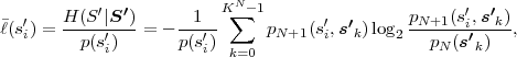 | (5.63) |
where k is an index that indicates any of the KN combinations of the last N output samples, p is the marginal pmf of the output samples, and pN and pN+1 are the joint pmfs for N and N + 1 successive output samples, respectively. It should be noted that the argument of the logarithm represents the conditional pmf for an output sample S′ given the N preceding output samples S′.
Each joint pmf for N successive output samples, including the marginal pmf p with N = 1, is determined by the joint pdf fN of the input source and the decision thresholds,
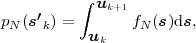 | (5.64) |
where uk and uk+1 represent the ordered sets of lower and upper interval boundaries for the vector s′k of output samples. Hence, the average codeword length (s′i) can be directly derived based on the joint pdf for the input process and the decision thresholds. In a similar way, the average codeword lengths for block codes of N samples can be approximated based on the block entropy for N successive output samples.
We now investigate the asymptotic operational distortion rate function
for high rates. If we again assume that we employ a conditional lossless
code that exploits the conditional pmf using the preceding N output
samples, the rate R can be approximated by the corresponding conditional
entropy H(Sn|Sn-1, ,Sn-N),
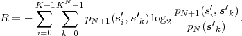 | (5.65) |
For small quantization intervals Δi (high rates), we can assume that the joint pdfs fN for the input sources are nearly constant inside each N-dimensional hypercube given by a combination of quantization intervals, which yields the approximations
 | (5.66) |
where Δk represents the Cartesian product of quantization interval sizes that are associated with the vector of reconstruction levels s′k. By inserting these approximations in (5.65), we obtain
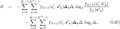
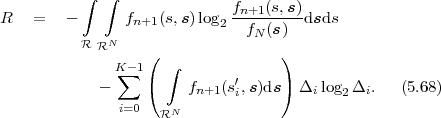
 ,Sn-N) for an input sample given the preceding N
input symbols and the second integral is the value f(s′i) of marginal pdf of
the input source. Using the high rate approximation p(s′i) = f(s′i)Δi, we
obtain
,Sn-N) for an input sample given the preceding N
input symbols and the second integral is the value f(s′i) of marginal pdf of
the input source. Using the high rate approximation p(s′i) = f(s′i)Δi, we
obtain
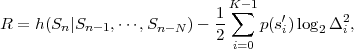 | (5.69) |
which is similar to (5.49). In the same way as for (5.49) in sec. 5.2.3, we can now apply Jensen’s inequality and then insert the high rate approximation (5.41) for the MSE distortion measure. As a consequence of Jensen’s inequality, we note that also for conditional lossless codes, the optimal quantizer design for high rates has uniform quantization steps sizes. The asymptotic operational distortion rate function for an optimum quantizer with conditional lossless codes is given by
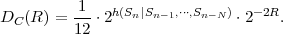 | (5.70) |
In comparison to the Gish & Pierce asymptote (5.52), the first-order differential entropy h(S) is replaced by the conditional entropy given the N preceding input samples.
In a similar way, we can also derive the asymptotic distortion rate function for block entropy codes (as the block Huffman code) of size N. We obtain the result that also for block entropy codes, the optimal quantizer design for high rates has uniform quantization step sizes. The corresponding asymptotic operational distortion rate function is
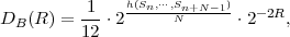 | (5.71) |
where h(Sn,…,Sn+N-1) denotes the joint differential entropy for N successive input symbols.
The achievable distortion rate function depends on the complexity of the applied lossless coding technique (which is basically given by the parameter N). For investigating the asymptotically achievable operational distortion rate function for arbitrarily complex entropy coding techniques, we take the limit for N →∞, which yields
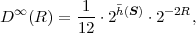 | (5.72) |
where (S) denotes the differential entropy rate of the input source. A comparison with the Shannon lower bound (4.65) shows that the asymptotically achievable distortion for high rates and arbitrarily complex entropy coding is 1.53 dB larger than the fundamental performance bound. The corresponding rate increase is 0.25 bit per sample. It should be noted that this asymptotic bound can only be achieved for high rates. Furthermore, in general, the entropy coding would require the storage of a very large set of codewords or conditional probabilities, which is virtually impossible in real applications.
The investigation of scalar quantization (SQ) showed that it is impossible to achieve the fundamental performance bound using a source coding system consisting of scalar quantization and lossless coding. For high rates the difference to the fundamental performance bound is 1.53 dB or 0.25 bit per sample. This gap can only be reduced if multiple samples are jointly quantized, i.e., by vector quantization (VQ). Although vector quantization is rarely used in video coding, we will give a brief overview in order to illustrate its design, performance, complexity, and the reason for the limitation of scalar quantization.
In N-dimensional vector quantization, an input vector s consisting of N
samples is mapped to a set of K reconstruction vectors {s′i}. We will
generally assume that the input vectors are blocks of N successive samples
of a realization of a stationary random process {S}. Similarly as for
scalar quantization, we restrict our considerations to regular vector
quantizers55 Regular quantizers are optimal with respect to the MSE distortion measure.
for which the quantization cells are convex
sets66 A set of points in  N is convex, if for any two points of the set, all points on the straight line
connecting the two points are also elements of the set.
and each reconstruction vector is an element of the associated quantization
cell. The average distortion and average rate of a vector quantizer are given
by (5.5) and (5.7), respectively.
N is convex, if for any two points of the set, all points on the straight line
connecting the two points are also elements of the set.
and each reconstruction vector is an element of the associated quantization
cell. The average distortion and average rate of a vector quantizer are given
by (5.5) and (5.7), respectively.
5.3.1 Vector Quantization with Fixed-Length Codes
We first investigate a vector quantizer design that minimizes the distortion D for a given quantizer size K, i.e., the counterpart of the Lloyd quantizer. The necessary conditions for the reconstruction vectors and quantization cells can be derived in the same way as for the Lloyd quantizer in sec. 5.2.1 and are given by
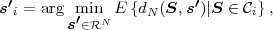 | (5.73) |
and
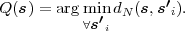 | (5.74) |
The extension of the Lloyd algorithm to vector quantization [46] is referred to as Linde-Buzo-Gray algorithm (LBG). For a sufficiently large training set {sn} and a given quantizer size K, the algorithm can be stated as follows:
i according to
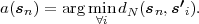

where the expectation value is taken over the training set.
Fig. 5.14 Illustration of the LBG algorithm for a quantizer with N = 2 and K = 16 and a Gaussian iid process with unit variance. The lines mark the boundaries of the quantization cells, the crosses show the reconstruction vectors, and the light-colored dots represent the samples of the training set.
An an example, we designed a 2-d vector quantizer for a Gaussian iid process with unit variance. The selected quantizer size is K = 16 corresponding to a rate of 2 bit per (scalar) sample. The chosen initialization as well as the obtained quantization cells and reconstruction vectors after the 8-th and 49-th iteration of the LBG algorithm are illustrated in Fig. 5.14. In Fig. 5.15, the distortion is plotted as function of the iteration step.
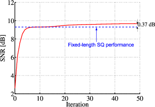
After the 8-th iteration, the 2-dimensional vector quantizer shows a similar distortion (9.30 dB) as the scalar Lloyd quantizer at the same rate of R = 2 bit per (scalar) sample. This can be explained by the fact that the quantization cells are approximately rectangular shaped and that such rectangular cells would also be constructed by a corresponding scalar quantizer (if we illustrate the result for 2 consecutive samples). After the 49-th iteration, the cells of the vector quantizer are shaped in a way that a scalar quantizer cannot create and the SNR is improved to 9.67 dB.
Fig. 5.16 Illustration of the LBG algorithm for a quantizer with N = 2 and K = 256 and a Gaussian iid process with unit variance: (left) resulting quantization cells and reconstruction vectors after 49 iterations; (right) distortion as function of the iteration step.
Fig. 5.16 shows the result of the LBG algorithm for a vector quantizer with N = 2 and K = 256, corresponding to a rate of R = 4 bit per sample, for the Gaussian iid source with unit variance. After the 49-th iteration, the gain for two-dimensional VQ is around 0.9 dB compared to SQ with fixed-length codes resulting in an SNR of 20.64 dB (of conjectured 21.05 dB [50]). The result indicates that at higher bit rates, the gain of VQ relative to SQ with fixed-length codes increases.
Fig. 5.17 Results of the LBG algorithm for a 2-d VQ with a size of K = 16 (top) and K = 256 (bottom) for a Laplacian iid source with unit variance.
Fig. 5.17 illustrates the results for a 2-d VQ design for a Laplacian iid source with unit variance and two different quantizer sizes K. For K = 16, which corresponds to a rate of R = 2 bit per sample, the SNR is 8.87 dB. Compared to SQ with fixed-length codes at the same rate, a gain of 1.32 dB has been achieved. For a rate of R = 4 bit per sample (K = 256), the SNR gain is increased to 1.84 dB resulting in an SNR of 19.4 dB (of conjectured 19.99 dB [50]).
5.3.2 Vector Quantization with Variable-Length Codes
For designing a vector quantizer with variable-length codes, we have to minimize the distortion D subject to a rate constraint, which can be effectively done using Lagrangian optimization. Following the arguments in sec. 5.2.2, it is justified to approximate the rate by the entropy H(Q(S)) of the output vectors and to set the average codeword lengths equal to (s′i) = -log 2p(s′i). Such a quantizer design is also referred to as entropy-constrained vector quantizer (ECVQ). The necessary conditions for the reconstruction vectors and quantization cells can be derived in the same way as for the entropy-constrained scalar quantizer (ECSQ) and are given by (5.73) and
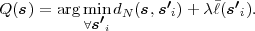 | (5.75) |
The extension of the entropy-constrained Lloyd algorithm to vector quantization [9] is also referred to as Chou-Lookabaugh-Gray algorithm (CLG). For a sufficiently large training set {sn} and a given Lagrange parameter λ, the CLG algorithm can be stated as follows:
i according to
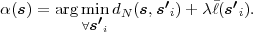
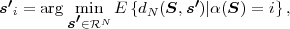
where the expectation value is taken over the training set.
As examples, we designed a 2-d ECVQ for a Gaussian and Laplacian iid process with unit variance and an average rate, measured as entropy, of R = 2 bit per sample. The results of the CLG algorithm are illustrated in Fig. 5.18. The SNR gain compared to an ECSQ design with the same rate is 0.26 dB for the Gaussian and 0.37 dB for the Laplacian distribution.
Fig. 5.18 Results of the CLG algorithm for a Gaussian (top) and Laplacian (bottom) iid source with unit variance and a rate (entropy) of R = 2 bit per sample. The dashed line in the diagrams on the right shows the distortion for an ECSQ design with the same rate.
5.3.3 The Vector Quantization Advantage
The examples for the LBG and CLG algorithms showed that vector quantization increases the coding efficiency compared to scalar quantization. According to the intuitive analysis in [52], the performance gain can be attributed to three different effects: the space filling advantage, the shape advantage, and the memory advantage. In the following, we will briefly explain and discuss these advantages. We will see that the space filling advantage is the only effect that can be exclusively achieved with vector quantization. The associated performance gain is bounded to 1.53 dB or 0.25 bit per sample. This bound is asymptotically achieved for large quantizer dimensions and large rates, and corresponds exactly to the gap between the operational rate distortion function for scalar quantization with arbitrarily complex entropy coding and the rate distortion bound at high rates. For a deeper analysis of the vector quantization advantages, the reader is referred to the discussion in [52] and the quantitative analysis in [50].
When we analyze the results of scalar quantization in higher dimension,
we see that the N-dimensional space is partitioned into N-dimensional
hyperrectangles (Cartesian products of intervals). This does however not
represent the densest packing in N. With vector quantization of
dimension N, we have extra freedom in choosing the shapes of the
quantization cells. The associated increase in coding efficiency is referred to
as space filling advantage.
The space filling advantage can be observed in the example for the LBG algorithm with N = 2 and a Gaussian iid process in Fig. 5.14. After the 8-th iteration, the distortion is approximately equal to the distortion of the scalar Lloyd quantizer with the same rate and the reconstruction cells are approximately rectangular shaped. However, the densest packing in two dimensions is achieved by hexagonal quantization cells. After the 49-th iteration of the LBG algorithm, the quantization cells in the center of the distribution look approximately like hexagons. For higher rates, the convergence toward hexagonal cells is even better visible as can be seen in Figs. 5.16 and 5.17
Fig. 5.19 Convergence of LBG algorithm with N = 2 toward hexagonal quantization cells for a uniform iid process.
To further illustrate the space filling advantage, he have conducted
another experiment for a uniform iid process with A = 10. The operational
distortion rate function for scalar quantization is given by D(R) =  2-2R.
For a scalar quantizer of size K = 10, we obtain a rate (entropy) of 3.32 bit
per sample and a distortion of 19.98 dB. The LBG design with N = 2 and
K = 100 is associated with about the same rate. The partitioning converges
toward a hexagonal lattice as illustrated in Fig. 5.19 and the SNR is
increased to 20.08 dB.
2-2R.
For a scalar quantizer of size K = 10, we obtain a rate (entropy) of 3.32 bit
per sample and a distortion of 19.98 dB. The LBG design with N = 2 and
K = 100 is associated with about the same rate. The partitioning converges
toward a hexagonal lattice as illustrated in Fig. 5.19 and the SNR is
increased to 20.08 dB.
The gain due to choosing the densest packing is independent of the source distribution or any statistical dependencies between the random variables of the input process. The space filling gain is bounded to 1.53 dB, which can be asymptotically achieved for high rates if the dimensionality of the vector quantizer approaches infinity [50].
Fig. 5.20 Shape advantage for Gaussian and Laplacian iid sources as function of the vector quantizer dimension N.
The shape advantage describes the effect that the quantization cells of optimal VQ designs adapt to the shape of the source pdf. In the examples for the CLG algorithm, we have however seen that, even though ECVQ provides a better performance than VQ with fixed-length code, the gain due to VQ is reduced if we employ variable-length coding for both VQ and SQ. When comparing ECVQ with ECSQ for iid sources, the gain of VQ reduces to the space filling advantage, while the shape advantage is exploited by variable-length coding. However, VQ with fixed-length codes can also exploit the gain that ECSQ shows compared to SQ with fixed-length codes [50].
The shape advantage for high rates has been estimated in [50]. Fig. 5.20 shows this gain for Gaussian and Laplacian iid random processes. In practice, the shape advantage is exploited by using scalar quantization in combination with entropy coding techniques such as Huffman coding or arithmetic coding.
For sources with memory, there are linear or nonlinear dependencies between the samples. In optimal VQ designs, the partitioning of the N-dimensional space into quantization cells is chosen in a way that these dependencies are exploited. This is illustrated in Fig. 5.21, which shows the ECVQ result of the CLG algorithm for N = 2 and a Gauss-Markov process with a correlation factor of ρ = 0.9 for two different values of the Lagrange parameter λ.
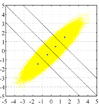
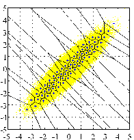
An quantitative estimation of the gain resulting from the memory advantage at high rates was done in [50]. Fig. 5.22 shows the memory gain for Gauss-Markov sources with different correlation factors as function of the quantizer dimension N.
Fig. 5.22 Memory gain as function of the quantizer dimension N for Gauss-Markov sources with different correlation factors ρ.
For sources with strong dependencies between the samples, such as video signals, the memory gain is much larger than the shape and space filling gain. In video coding, a suitable exploitation of the statistical dependencies between samples is one of the most relevant design aspects. The linear dependencies between samples can also be exploited by combining scalar quantization with linear prediction or linear transforms. These techniques are discussed in chapters 6 and 7. By combining scalar quantization with advanced entropy coding techniques, which we discussed in sec. 5.2.6, it is possible to partially exploit both linear as well as nonlinear dependencies.
5.3.4 Performance and Complexity
For further evaluating the performance of vector quantization, we compared the operational rate distortion functions for CLG designs with different quantizer dimensions N to the rate distortion bound and the operational distortion functions for scalar quantizers with fixed-length and variable-length77 In this comparison, it is assumed that the dependencies between the output samples or output vectors are not exploited by the applied lossless coding. codes. The corresponding rate distortion curves for a Gauss-Markov process with a correlation factor of ρ = 0.9 are depicted in Fig. 5.23. For quantizers with fixed-length codes, the rate is given the binary logarithm of the quantizer size K; for quantizers with variable-length codes, the rate is measured as the entropy of the reconstruction levels or reconstruction vectors.
Fig. 5.23 Estimated vector quantization advantage at high rates [50] for a Gauss-Markov source with a correlation factor of ρ = 0.9.
The operational distortion rate curves for vector quantizers of dimensions N = 2,5,10, and 100, labeled with “VQ, K = N(e)”, show the theoretical performance for high rates, which has been estimated in [50]. These theoretical results have been verified for N = 2 by designing entropy-constrained vector quantizers using the CLG algorithm. The theoretical vector quantizer performance for a quantizer dimension of N = 100 is very close to the distortion rate function of the investigated source. In fact, vector quantization can asymptotically achieve the rate distortion bound as the dimension N approaches infinity. Moreover, vector quantization can be interpreted as the most general lossy source coding system. Each source coding system that maps a vector of N samples to one of K codewords (or codeword sequences) can be designed as vector quantizer of dimension N and size K.
Despite the excellent coding efficiency vector quantization is rarely used in video coding. The main reason is the associated complexity. On one hand, a general vector quantizer requires the storage of a large codebook. This issue becomes even more problematic for systems that must be able to encode and decode sources at different bit rates, as it is required for video codecs. On the other hand, the computationally complexity for associating an input vector with the best reconstruction vector in rate distortion sense is very large in comparison to the encoding process for scalar quantization that is used in practice. One way to reduce the requirements on storage and computational complexity is to impose structural constraints on the vector quantizer. Examples for such structural constraints include:
In particular, predictive VQ can be seen as a generalization of a number of very popular techniques including motion compensation in video coding. For the actual quantization, video codecs mostly include a simple scalar quantizer with uniformly distributed reconstruction levels (sometimes with a deadzone around zero), which is combined with entropy coding and techniques such as linear prediction or linear transforms in order to exploit the shape of the source distribution and the statistical dependencies of the source. For video coding, the complexity of vector quantizers including those with structural constraints is considered as too large in relation to the achievable performance gains.
In this chapter, we have discussed quantization starting with scalar quantizers. The Lloyd quantizer that is constructed using an iterative procedure provides the minimum distortion for a given number of reconstruction levels. It is the optimal quantizer design if the reconstruction levels are transmitted using fixed-length codes. The extension of the quantizer design for variable-length codes is achieved by minimizing the distortion D subject to a rate constraint R < Rmax, which can be formulated as a minimization of a Lagrangian functional D + λR. The corresponding iterative design algorithm includes a sufficiently accurate estimation of the codeword lengths that are associated with the reconstruction levels. Usually the codeword lengths are estimated based on the entropy of the output signal, in which case the quantizer design is also referred to as entropy-constrained Lloyd quantizer.
At high rates, the operational distortion rate functions for scalar quantization with fixed- and variable-length codes as well as the Shannon lower bound can be described by
 | (5.76) |
where X either indicates the Shannon lower bound or scalar quantization with fixed- or variable-length codes. For a given X, the factors εX2 depend only of the statistical properties of the input source. If the output samples are coded with an arbitrarily complex entropy coding scheme, the difference between the operational distortion rate function for optimal scalar quantization and the Shannon lower bound is 1.53 dB or 0.25 bit per sample at high rates. Another remarkable result is that at high rates, optimal scalar quantization with variable-length codes is achieved if all quantization intervals have the same size.
In the second part of the chapter, we discussed the extension of scalar quantization to vector quantization, by which the rate distortion bound can be asymptotically achieved as the quantizer dimension approaches infinity. The coding efficiency improvements of vector quantization relative to scalar quantization can be attributed to three different effects: the space filling advantage, the shape advantage, and the memory advantage. While the space filling advantage can be only achieved by vector quantizers, the shape and memory advantage can also be exploited by combining scalar quantization with a suitable entropy coding and techniques such as linear prediction and linear transforms.
Despite its superior rate distortion performance, vector quantization is rarely used in video coding applications because of its complexity. Instead, modern video codecs combine scalar quantization with entropy coding, linear prediction, and linear transforms in order to achieve a high coding efficiency at a moderate complexity level.
This is the html version of the book:
Thomas Wiegand and Heiko Schwarz (2010): "Source Coding: Part I of Fundamentals of Source and Video Coding", Now Publishers, Foundations and Trends® in Signal Processing: Vol. 4: No 1-2, pp 1-222. (pdf version of the book)
6 Predictive Coding
In the previous chapter, we investigated the design and rate distortion performance of quantizers. We showed that the fundamental rate distortion bound can be virtually achieved by unconstrained vector quantization of a sufficiently large dimension. However, due to the very large amount of data in video sequences and the real-time requirements that are found in most video coding applications, only low-complex scalar quantizers are typically used in this area. For iid sources, the achievable operational rate distortion function for high rate scalar quantization lies at most 1.53 dB or 0.25 bit per sample above the fundamental rate distortion bound. This represents a suitable trade-off between coding efficiency and complexity. But if there is a large amount of dependencies between the samples of an input signal, as it is the case in video sequences, the rate distortion performance for simple scalar quantizers becomes significantly worse than the rate distortion bound. A source coding system consisting of a scalar quantizer and an entropy coder can exploit the statistical dependencies in the input signal only if the entropy coder uses higher-order conditional or joint probability models. The complexity of such an entropy coder is however close to that of a vector quantizer, so that such a design is unsuitable in practice. Furthermore, video sequences are highly nonstationary and conditional or joint probabilities for nonstationary sources are typically very difficult to estimate accurately. It is desirable to combine scalar quantization with additional tools that can efficiently exploit the statistical dependencies in a source at a low complexity level. One of such coding concepts is predictive coding, which we will investigate in this chapter. The concepts of prediction and predictive coding are widely used in modern video coding. Well-known examples are intra prediction, motion-compensated prediction, and motion vector prediction.
The basic structure of predictive coding is illustrated in Fig. 6.1 using the notation of random variables. The source samples {sn} are not directly quantized. Instead, each sample sn is predicted based on previous samples. The prediction value ŝn is subtracted from the value of the input sample sn yielding a residual or prediction error sample un = sn -ŝn. The residual sample un is then quantized using scalar quantization. The output of the quantizer is a reconstructed value u′n for the residual sample un. At the decoder side, the reconstruction u′n of the residual sample is added to the predictor ŝn yielding the reconstructed output sample s′n = ŝn + u′n.
Intuitively, we can say that the better the future of a random process is predicted from its past and the more redundancy the random process contains, the less new information is contributed by each successive observation of the process. In the context of predictive coding, the predictors ŝn should be chosen in a way that they can be easily computed and result in a rate distortion efficiency of the predictive coding system that is as close as possible to the rate distortion bound.
In this chapter, we discuss the design of predictors with the emphasis on linear predictors and analyze predictive coding systems. For further details, the reader is referred to the classic tutorial [51], and the detailed treatments in [75] and [24].
Prediction is a statistical estimation procedure where the value of a
particular random variable Sn of a random process {Sn} is estimated
based on the values of other random variables of the process. Let n be a
set of observed random variables. As a typical example, the observation set
can represent the N random variables n = {Sn-1,Sn-2, ,Sn-N} that
precede that random variable Sn to be predicted. The predictor for the
random variable Sn is a deterministic function of the observation set n
and is denoted by An(n). In the following, we will omit this functional
notation and consider the prediction of a random variable Sn as another
random variable denoted by Ŝn,
,Sn-N} that
precede that random variable Sn to be predicted. The predictor for the
random variable Sn is a deterministic function of the observation set n
and is denoted by An(n). In the following, we will omit this functional
notation and consider the prediction of a random variable Sn as another
random variable denoted by Ŝn,
 | (6.1) |
The prediction error or residual is given by the difference of the random variable Sn to be predicted and its prediction Ŝn. It can also be interpreted as a random variable and is be denoted Un,
 | (6.2) |
If we predict all random variables of a random process {Sn}, the sequence of predictions {Ŝn} and the sequence of residuals {Un} are random processes. The prediction can then be interpreted as a mapping of an input random process {Sn} to an output random process {Un} representing the sequence of residuals as illustrated in Fig. 6.2.
In order to derive optimum predictors, we have to discuss first how the goodness of a predictor can be evaluated. In the context of predictive coding, the ultimate goal is to achieve the minimum distortion between the original and reconstructed samples subject to a given maximum rate. For the MSE distortion measure (or in general for all additive difference distortion measures), the distortion between a vector of N input samples s and the associated vector of reconstructed samples s′ is equal to the distortion between the corresponding vector of residuals u and the associated vector of reconstructed residuals u′,
 | (6.3) |
Hence, the operational distortion rate function of a predictive coding
systems is equal to the operational distortion rate function for scalar
quantization of the prediction residuals. As stated in sec. 5.2.4, the
operational distortion rate curve for scalar quantization of the residuals can
be stated as D(R) = σU2 ⋅ g(R), where σU2 is the variance of the residuals
and the function g(R) depends only on the type of the distribution of the
residuals. Hence, the rate distortion efficiency of a predictive coding
system depends on the variance of the residuals and the type of their
distribution. We will neglect the dependency on the distribution type
and define that a predictor An(n) given an observation set n is
optimal if it minimizes the variance σU2 of the prediction error.
In the literature [51, 75, 24], the most commonly used criterion
for the optimality of a predictor is the minimization of the MSE
between the input signal and its prediction. This is equivalent to the
minimization of the second moment ϵU2 = σU2 + μU2, or the energy, of the
prediction error signal. Since the minimization of the second moment ϵU2
implies11 We will later prove this statement for linear prediction.
a minimization of the variance σU2 and the mean μU, we will also consider
the minimization of the mean squared prediction error ϵU2.
When considering the more general criterion of the mean squared
prediction error, the selection of the optimal predictor An(n) given an
observation set n is equivalent to the minimization of
 | (6.4) |
The solution to this minimization problem is given by the conditional mean
of the random variable Sn given the observation set n,
 | (6.5) |
This can be proved by using the formulation
Since E and An(n) are deterministic functions given the
observation set n, we can write
and An(n) are deterministic functions given the
observation set n, we can write 
 = E
= E ,
which was derived in (2.32), we obtain for the cross term in (6.6),
,
which was derived in (2.32), we obtain for the cross term in (6.6),
 | (6.9) |
which proves that the conditional mean E minimizes the mean
squared prediction error for a given observation set n.
minimizes the mean
squared prediction error for a given observation set n.
We will show later that in predictive coding the observation set n must
consist of reconstructed samples. If we for example use the last N
reconstructed samples as observation set, n = {S′n-1, ,S′n-N}, it is
conceptually possible to construct a table in which the conditional
expectations E
,S′n-N}, it is
conceptually possible to construct a table in which the conditional
expectations E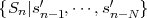 are stored for all possible combinations
of the values of s′n-1 to s′n-N. This is in some way similar to scalar
quantization with an entropy coder that employs the conditional
probabilities p(sn|s′n-1,
are stored for all possible combinations
of the values of s′n-1 to s′n-N. This is in some way similar to scalar
quantization with an entropy coder that employs the conditional
probabilities p(sn|s′n-1, ,s′n-N) and does not significantly reduce the
complexity. For obtaining a low-complexity alternative to this scenario, we
have to introduce structural constraints for the predictor An(n). Before we
state a reasonable structural constraint, we derive the optimal predictors
according to (6.5) for two examples.
,s′n-N) and does not significantly reduce the
complexity. For obtaining a low-complexity alternative to this scenario, we
have to introduce structural constraints for the predictor An(n). Before we
state a reasonable structural constraint, we derive the optimal predictors
according to (6.5) for two examples.
As a first example, we consider a stationary Gaussian source and
derive the optimal predictor for a random variable Sn given a vector
Sn-k = (Sn-k, ,Sn-k-N+1)T , with k > 0, of N preceding samples. The
conditional distribution f(Sn|Sn-k) of jointly Gaussian random variables is
also Gaussian. The conditional mean E
,Sn-k-N+1)T , with k > 0, of N preceding samples. The
conditional distribution f(Sn|Sn-k) of jointly Gaussian random variables is
also Gaussian. The conditional mean E and thus the optimal
predictor is given by (see for example [26])
and thus the optimal
predictor is given by (see for example [26])
 | (6.10) |
where μS represents the mean of the Gaussian process, eN is the N-dimensional vector with all elements equal to 1, and CN is the N-th order autocovariance matrix, which is given by
 | (6.11) |
The vector ck is an autocovariance vector and is given by
 | (6.12) |
Autoregressive processes are an important model for random sources. An autoregressive process of order m, also referred to as AR(m) process, is given by the recursive formula
where μS is the mean of the random process, am = (a1, ,am)T is a
constant parameter vector, and {Zn} is a zero-mean iid process. We
consider the prediction of a random variable Sn given the vector Sn-1 of
the N directly preceding samples, where N is greater than or equal
to the order m. The optimal predictor is given by the conditional
mean E
,am)T is a
constant parameter vector, and {Zn} is a zero-mean iid process. We
consider the prediction of a random variable Sn given the vector Sn-1 of
the N directly preceding samples, where N is greater than or equal
to the order m. The optimal predictor is given by the conditional
mean E . By defining an N-dimensional parameter vector
aN = (a1,
. By defining an N-dimensional parameter vector
aN = (a1, ,am,0,
 ,0)T , we obtain
For both considered examples, the optimal predictor is given by a linear function of the observation vector. In a strict sense, it is an affine function if the mean μ of the considered processes is nonzero. If we only want to minimize the variance of the prediction residual, we do not need the constant offset and can use strictly linear predictors. For predictive coding systems, affine predictors have the advantage that the scalar quantizer can be designed for zero-mean sources. Due to their simplicity and their effectiveness for a wide range of random processes, linear (and affine) predictors are the most important class of predictors for video coding applications. It should however be noted that nonlinear dependencies in the input process cannot be exploited using linear or affine predictors. In the following, we will concentrate on the investigation of linear prediction and linear predictive coding.
In the following, we consider linear and affine prediction of a random
variable Sn given an observation vector Sn-k = [Sn-k, ,Sn-k-N+1]T ,
with k > 0, of N preceding samples. We restrict our considerations to
stationary processes. In this case, the prediction function An(Sn-k) is
independent of the time instant of the random variable to be predicted and
is denoted by A(Sn-k). For the more general affine form, the predictor is
given by
,Sn-k-N+1]T ,
with k > 0, of N preceding samples. We restrict our considerations to
stationary processes. In this case, the prediction function An(Sn-k) is
independent of the time instant of the random variable to be predicted and
is denoted by A(Sn-k). For the more general affine form, the predictor is
given by
 | (6.15) |
where the constant vector hN = (h1, ,hN)T and the constant offset h0
are the parameters that characterize the predictor. For linear predictors, the
constant offset h0 is equal to zero.
,hN)T and the constant offset h0
are the parameters that characterize the predictor. For linear predictors, the
constant offset h0 is equal to zero.
The variance σU2 of the prediction residual depends on the predictor parameters and can be written as
The constant offset h0 has no influence on the variance of the residual. The variance σU2 depends only on the parameter vector hN. By further reformulating the expression (6.16), we obtain where σS2 is the variance of the input process and CN and ck are the autocovariance matrix and the autocovariance vector of the input process given by (6.11) and (6.12), respectively.The mean squared prediction error is given by
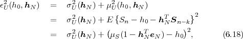
 | (6.19) |
This selection of h0 yields a mean of μU = 0 for the prediction error signal, and the MSE between the input signal and the prediction ϵU2 is equal to the variance of the prediction residual σU2. Due to this simple relationship, we restrict the following considerations to linear predictors
 | (6.20) |
and the minimization of the variance σU2. But we keep in mind that the affine predictor that minimizes the mean squared prediction error can be obtained by additionally selecting an offset h0 according to (6.19). The structure of a linear predictor is illustrated in Fig. 6.3.
A linear predictor is called an optimal linear predictor if its parameter vector hN minimizes the variance σU2(hN) given in (6.17). The solution to this minimization problem can be obtained by setting the partial derivatives of σU2 with respect to the parameters hi, with 1 ≤ i ≤ N, equal to 0. This yields the linear equation system
 | (6.21) |
We will prove later that this solution minimizes the variance σU2. The N equations of the equation system (6.21) are also called the normal equations or the Yule-Walker equations. If the autocorrelation matrix CN is nonsingular, the optimal parameter vector is given by
 | (6.22) |
The autocorrelation matrix CN of a stationary process is singular if and
only if N successive random variables Sn,Sn+1, ,Sn+N-1 are linearly
dependent (see [75]), i.e., if the input process is deterministic. We ignore
this case and assume that CN is always nonsingular.
,Sn+N-1 are linearly
dependent (see [75]), i.e., if the input process is deterministic. We ignore
this case and assume that CN is always nonsingular.
By inserting (6.22) into (6.17), we obtain the minimum prediction error variance
Note that (hN*)T = ckT CN-1 follows from that fact that the autocorrelation matrix CN and thus also its inverse CN-1 is symmetric.We now prove that the solution given by the normal equations (6.21) indeed minimizes the prediction error variance. Therefore, we investigate the prediction error variance for an arbitrary parameter vector hN, which can be represented as hN = hN* + δN. Inserting this relationship into (6.17) and using (6.21) yields
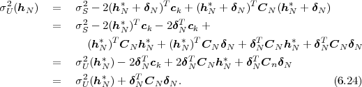
 of the random variable δNT Sn and is thus
always greater than or equal to 0. Hence, we have
of the random variable δNT Sn and is thus
always greater than or equal to 0. Hence, we have
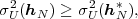 | (6.25) |
which proves that (6.21) specifies the parameter vector hN* that minimizes the prediction error variance.
In the following, we derive another important property for optimal linear predictors. We consider the more general affine predictor and investigate the correlation between the observation vector Sn-k and the prediction residual Un,
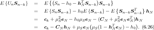
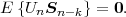 | (6.27) |
Hence, optimal affine prediction yields a prediction residual Un that is uncorrelated with the observation vector Sn-k. For optimal linear predictors, equation (6.27) holds only for zero-mean input signals. In general, only the covariance between the prediction residual and each observation is equal to zero,
 | (6.28) |
The linear prediction for a single random variable Sn given an
observation vector Sn-k can also be extended to the prediction of a vector
Sn+K-1 = (Sn+K-1,Sn+K-2, ,Sn)T of K random variables. For each
random variable of Sn+K-1, the optimal linear or affine predictor can be
derived as discussed above. If the parameter vectors hN are arranged in a
matrix and the offsets h0 are arranged in a vector, the prediction can be
written as
,Sn)T of K random variables. For each
random variable of Sn+K-1, the optimal linear or affine predictor can be
derived as discussed above. If the parameter vectors hN are arranged in a
matrix and the offsets h0 are arranged in a vector, the prediction can be
written as
 | (6.29) |
where HK is an K ×N matrix whose rows are given by the corresponding parameter vectors hN and hK is a K-dimensional vector whose elements are given by the corresponding offsets h0.
The most often used prediction is the one-step prediction in which
a random variable Sn is predicted using the N directly preceding
random variables Sn-1 = (Sn-1, ,Sn-N)T . For this case, we now
derive some useful expressions for the minimum prediction error
variance σU2(hN*), which will be used later for deriving an asymptotic
bound.
,Sn-N)T . For this case, we now
derive some useful expressions for the minimum prediction error
variance σU2(hN*), which will be used later for deriving an asymptotic
bound.
For the one-step prediction, the normal equations (6.21) can be written in matrix notation as
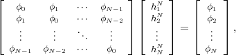 | (6.30) |
where the factors hkN represent the elements of the optimal parameter
vector hN* = (h1N, ,hNN)T for linear prediction using the N preceding
samples. The covariances E
,hNN)T for linear prediction using the N preceding
samples. The covariances E are
denoted by ϕk. By adding a matrix column to the left, multiplying the
parameter vector hN* with -1, and adding an element equal to 1 at the
top of the parameter vector, we obtain
are
denoted by ϕk. By adding a matrix column to the left, multiplying the
parameter vector hN* with -1, and adding an element equal to 1 at the
top of the parameter vector, we obtain
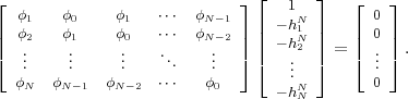 | (6.31) |
We now include the expression for the minimum prediction variance into the matrix equation. The prediction error variance for optimal linear prediction using the N preceding samples is denoted by σN2. Using (6.23) and (6.22), we obtain
 | (6.32) |
Adding this relationship to the matrix equation (6.31) yields
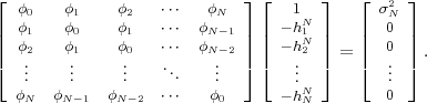 | (6.33) |
This equation is also referred to as the augmented normal equation.
It should be noted that the matrix on the left represents the
autocovariance matrix CN+1. We denote the modified parameter vector by
aN = (1,-h1N, ,-hNN)T . By multiplying both sides of (6.33) from the
left with the transpose of aN, we obtain
,-hNN)T . By multiplying both sides of (6.33) from the
left with the transpose of aN, we obtain
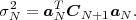 | (6.34) |
We have one augmented normal equation (6.33) for each particular number N of preceding samples in the observation vector. Combing the equations for 0 to N preceding samples into one matrix equation yields
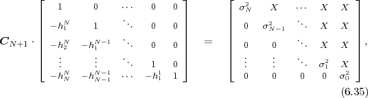
 | (6.36) |
Note that the determinant of a triangular matrix is the product of the elements on its main diagonal. Hence, the prediction error variance σN2 for optimal linear prediction using the N preceding samples can also be written as
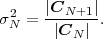 | (6.37) |
6.3.2 One-Step Prediction for Autoregressive Processes
In the following, we consider the particularly interesting case of optimal linear one-step prediction for autoregressive processes. As stated in sec. 6.1, an AR(m) process with the mean μS is defined by
 | (6.38) |
where {Zn} is a zero-mean iid process and am = (a1, ,am)T is a constant
parameter vector. We consider the one-step prediction using the N
preceding samples and the prediction parameter vector hN. We
assume that the number N of preceding samples in the observation
vector Sn-1 is greater than or equal to the process order m and define
a vector aN = (a1,
,am)T is a constant
parameter vector. We consider the one-step prediction using the N
preceding samples and the prediction parameter vector hN. We
assume that the number N of preceding samples in the observation
vector Sn-1 is greater than or equal to the process order m and define
a vector aN = (a1, ,am,0,
 ,0)T whose first m elements are
given by the process parameter vector am and whose last N - m
elements are equal to 0. The prediction residual can then be written
as
,0)T whose first m elements are
given by the process parameter vector am and whose last N - m
elements are equal to 0. The prediction residual can then be written
as
 | (6.39) |
By subtracting the mean E we obtain
 | (6.40) |
According to (6.28), the covariances between the residual Un and the random variables of the observation vector must be equal to 0 for optimal linear prediction. This gives
Since {Zn} is an iid process, Zn is independent of the past Sn-k, and the expectation value in (6.41) is equal to 0. The optimal linear predictor is given by
 | (6.42) |
Hence, for AR(m) processes, optimal linear prediction can be achieved by using the m preceding samples as observation vector and setting the prediction parameter vector hm equal to the parameter vector am of the AR(m) process. An increase of the prediction order N does not result in a decrease of the prediction error variance. All prediction parameters hk with k > m are equal to 0. It should be noted that if the prediction order N is less than the process order m, the optimal prediction coefficients hk are in general not equal to the corresponding process parameters ak. In that case, the optimal prediction vector must be determined according to the normal equations (6.21).
If the prediction order N is greater than or equal to the process order m, the prediction residual becomes
 | (6.43) |
The prediction residual is an iid process. Consequently, optimal linear
prediction of AR(m) processes with a prediction order N greater than or
equal to the process order m yields an iid residual process {Un} (white
noise) with a mean μU and a variance σU2 = E .
.
A Gauss-Markov process is a particular AR(1) process,
 | (6.44) |
for which the iid process {Zn} has a Gaussian distribution. It is completely characterized by its mean μS, its variance σS2, and the correlation coefficient ρ with -1 < ρ < 1. According to the analysis above, the optimal linear predictor for Gauss-Markov processes consists of a single coefficient h1 that is equal to ρ. The obtained prediction residual process {Un} represents white Gaussian noise with a mean μU = μS(1 - ρ) and a variance
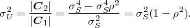 | (6.45) |
For measuring the effectiveness of a prediction often the prediction gain GP is used, which can be defined as the ratio of the signal variance and the variance of the prediction residual,
 | (6.46) |
For a fixed prediction structure, the prediction gain for optimal linear prediction does only depend on the autocovariances of the sources process. The prediction gain for optimal linear one-step prediction using the N preceding samples is given by
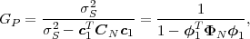 | (6.47) |
where ΦN = CN∕σS2 and ϕi = c1∕σS2 are the normalized autocovariance matrix and the normalized autocovariance vector, respectively.
The prediction gain for the one-step prediction of Gauss-Markov processes with a prediction coefficient h1 is given by
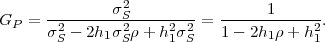 | (6.48) |
For optimal linear one-step prediction (h1 = ρ), we obtain
 | (6.49) |
For demonstrating the impact of choosing the prediction coefficient h1 for the linear one-step prediction of Gauss-Markov sources, Fig. 6.4 shows the prediction error variance and the prediction gain for a linear predictor with a fixed prediction coefficient of h1 = 0.5 and for the optimal linear predictor (h1 = ρ) as function of the correlation factor ρ.
Fig. 6.4 Linear one-step prediction for Gauss-Markov processes with unit variance. The diagrams show the prediction error variance (left) and the prediction gain (right) for a linear predictor with h1 = 0.5 (blues curve) and an optimal linear predictor with h1 = ρ (red curves) in dependence of the correlation factor ρ.
6.3.4 Asymptotic Prediction Gain
In the previous sections, we have focused on linear and affine prediction
with a fixed-length observation vector. Theoretically, we can make the
prediction order N very large and for N approaching infinity we
obtain an upper bound for the prediction gain. For deriving this
bound, we consider the one-step prediction of a random variable
Sn given the countably infinite set of preceding random variables
{Sn-1,Sn-2, }. For affine prediction, the prediction residual can be
written as
}. For affine prediction, the prediction residual can be
written as
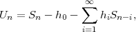 | (6.50) |
where the set {h0,h1, } is a countably infinite set of prediction
coefficients. According to the orthogonality condition (6.27), the prediction
residual Un is uncorrelated with all preceding random variables Sn-k with
k > 0. In addition, each prediction residual Un-k with k > 0 is completely
determined by a linear combination (6.50) of the random variables Sn-k-i
with i ≥ 0. Consequently, Un is also uncorrelated with the preceding
prediction residuals Un-k with k > 0. Hence, if the prediction order N
approaches infinity, the generated sequence of prediction residuals {Un}
represents an uncorrelated sequence. Its power spectral density is given
by
} is a countably infinite set of prediction
coefficients. According to the orthogonality condition (6.27), the prediction
residual Un is uncorrelated with all preceding random variables Sn-k with
k > 0. In addition, each prediction residual Un-k with k > 0 is completely
determined by a linear combination (6.50) of the random variables Sn-k-i
with i ≥ 0. Consequently, Un is also uncorrelated with the preceding
prediction residuals Un-k with k > 0. Hence, if the prediction order N
approaches infinity, the generated sequence of prediction residuals {Un}
represents an uncorrelated sequence. Its power spectral density is given
by
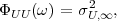 | (6.51) |
where σU,∞2 denotes the asymptotic one-step prediction error variance for N approaching infinity.
For deriving an expression for the asymptotic one-step prediction error variance σU,∞2, we restrict our considerations to zero-mean input processes, for which the autocovariance matrix CN is equal to the corresponding autocorrelation matrix RN, and first consider the limit
 | (6.52) |
Since the determinant of a N ×N matrix is given by the product of its
eigenvalues ξi(N), with i = 0,1, ,N - 1, we can write
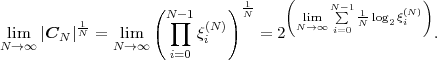 | (6.53) |
By applying Grenander and Szegö’s theorem for sequences of Toeplitz matrices (4.76), we obtain
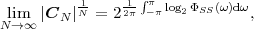 | (6.54) |
where ΦSS(ω) denotes the power spectral density of the input process {Sn}. As a further consequence of the convergence of the limit in (6.52), we can state
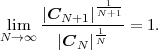 | (6.55) |
According to (6.37), we can express the asymptotic one-step prediction error variance σU,∞2 by
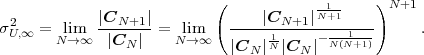 | (6.56) |
Applying (6.54) and (6.55) yields
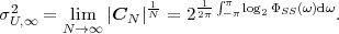 | (6.57) |
Hence, the asymptotic linear prediction gain for zero-mean input sources is given by
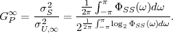 | (6.58) |
Fig. 6.5 Prediction gain for zero-mean Gauss-Markov sources: (left) Power spectral density; (right) Prediction gain.
It should be noted that for zero-mean AR(m) processes, such as zero-mean Gauss-Markov processes, this asymptotic prediction gain is already achieved by using optimal linear one-step predictors of a finite order N ≥ m. As an example, we know from (4.77) to (4.79) that
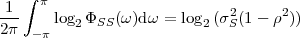 | (6.59) |
for Gauss-Markov processes. This yields the asymptotic prediction gain GP ∞ = 1∕(1 - ρ2), which we have already derived for the optimal one-step prediction in (6.45). This relationship can also be obtained by inserting the expression (2.50) for the determinant |CN| into (6.57). Fig. 6.5 illustrates the power spectral density and the prediction gain for stationary zero-mean Gauss-Markov processes.
6.4 Differential Pulse Code Modulation (DPCM)
In the previous sections, we investigated the prediction and in particular the linear prediction of a random variable Sn using the values of preceding random variables. We now consider the combination of prediction and scalar quantization.
We first consider the case that the random variables of the input process are predicted as discussed in the previous sections (i.e., using the original values of preceding samples) and the resulting prediction residuals are quantized. For the example of one-step prediction using the directly preceding sample, we obtain the encoder reconstructions
 | (6.60) |
At the decoder side, however, we do not know the original sample values. Here we must use the reconstructed values for deriving the prediction values. The corresponding decoder reconstructions are given by
 | (6.61) |
For such an open-loop predictive coding structure, the encoder and decoder reconstructions S′n,e and S′n,d differ by P(Sn-1) - P(S′n-1,d). If we use a recursive prediction structure as in the considered one-step prediction, the differences between encoder and decoder reconstructions increase over time. This effect is also referred to as drift and can only be avoided if the prediction at both encoder and decoder side uses reconstructed samples.
Fig. 6.6 Closed-loop predictive coding: (left) Prediction structure using reconstructed samples for forming the prediction signal; (right) DPCM structure.
The basic structure of a predictor that uses reconstructed samples S′n for forming the prediction signal is shown in the left block diagram of Fig. 6.6. This structure is also referred to as closed-loop predictive coding structure and is used in basically all video coding applications. The closed-loop structure ensures that a decoder can obtain the same reconstruction values as the encoder. By redrawing the block diagram without changing the signal flow we obtain the structure shown in the right block diagram of Fig. 6.6, which is also referred to as differential pulse code modulation (DPCM).
If we decompose the quantizer Q in Fig. 6.6 into an encoder mapping α that maps the prediction residuals Un onto quantization indexes In and a decoding mapping β that maps the quantization indexes In onto reconstructed residuals U′n and add a lossless coding γ for mapping the quantization indexes In onto codewords Bn, we obtain the well-known structure of a DPCM encoder shown on the left side of Fig. 6.7. The corresponding DPCM decoder is shown on the right side of Fig. 6.7. It includes, the inverse lossless coding γ-1, the decoder mapping β, and the predictor. If the codewords are transmitted over an error-free channel, the reconstruction values at the decoder side are identical to the reconstruction values at the encoder side, since the mapping of the quantization indexes In to reconstructed values S′n is the same in both encoder and decoder. The DPCM encoder contains the DPCM decoder except for the inverse lossless coding γ-1.
6.4.1 Linear Prediction for DPCM
In sec. 6.3, we investigated optimal linear prediction of a random
variable Sn using original sample values of the past. However, in DPCM
coding, the prediction Ŝn for a random variable Sn must be generated by a
linear combination of the reconstructed values S′n of already coded
samples. If we consider linear one-step prediction using an observation
vector S′n-1 = (S′n-1, ,S′n-N)T that consists of the reconstruction
values of the N directly preceding samples, the prediction value Ŝn can be
written as
,S′n-N)T that consists of the reconstruction
values of the N directly preceding samples, the prediction value Ŝn can be
written as
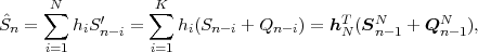 | (6.62) |
where Qn = U′n - Un denotes the quantization error, hN is the vector of
prediction parameters, Sn-1 = (Sn-1, ,Sn-N)T is the vector of the N
original sample values that precede the current sample Sn to be predicted,
and Qn-1 = (Qn-1,
,Sn-N)T is the vector of the N
original sample values that precede the current sample Sn to be predicted,
and Qn-1 = (Qn-1, ,Qn-N)T is the vector of the quantization errors for
the N preceding samples. The variance σU2 of the prediction residual Un
is given by
,Qn-N)T is the vector of the quantization errors for
the N preceding samples. The variance σU2 of the prediction residual Un
is given by
For high rates, the reconstructed samples S′n are a close approximation of the original samples Sn, and the optimal prediction parameter vector hN for linear prediction using reconstructed sample values is virtually identical to the optimal prediction parameter vector for linear prediction using original sample values. In the following, we concentrate on DPCM systems for which the linear prediction parameter vector is optimized for a prediction using original sample values, but we note that such DPCM systems are suboptimal for low rates.
As an important example, we investigate the rate distortion efficiency of linear predictive coding for stationary Gauss-Markov sources,
 | (6.64) |
We have shown in sec. 6.3.2 that the optimal linear predictor using original sample values is the one-tap predictor for which the prediction coefficient h1 equal to the correlation coefficient ρ of the Gauss-Markov process. If we use the same linear predictor with reconstructed samples, the prediction Ŝn for a random variable Sn can be written as
 | (6.65) |
where Qn-1 = U′n-1 - Un-1 denotes the quantization error. The prediction residual Un is given by
 | (6.66) |
For the prediction error variance σU2, we obtain
where σZ2 = E denotes the variance of the innovation process {Zn}
and σQ2 = E
denotes the variance of the innovation process {Zn}
and σQ2 = E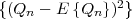 denotes the variance of the quantization
errors. Since {Zn} is an iid process and thus Zn is independent of the past
quantization errors Qn-1, the middle term in (6.67) is equal to 0.
Furthermore, as shown in sec. 2.3.1, the variance σZ2 of the innovation
process is given by σS2(1 - ρ2). Hence, we obtain
denotes the variance of the quantization
errors. Since {Zn} is an iid process and thus Zn is independent of the past
quantization errors Qn-1, the middle term in (6.67) is equal to 0.
Furthermore, as shown in sec. 2.3.1, the variance σZ2 of the innovation
process is given by σS2(1 - ρ2). Hence, we obtain
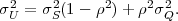 | (6.68) |
We further note that the quantization error variance σQ2 represents the distortion D of the DPCM quantizer and is a function of the rate R. As explained in sec. 5.2.4, we can generally express the distortion rate function of scalar quantizers by
 | (6.69) |
where σU2(R) represents the variance of the signal that is quantized. The function g(R) represents the operational distortion rate function for quantizing random variables that have the same distribution type as the prediction residual Un, but unit variance. Consequently, the variance of the prediction residual is given by
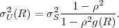 | (6.70) |
Using (6.69), we obtain the following operational distortion rate function for linear predictive coding of Gauss-Markov processes with a one-tap predictor for which the prediction coefficient h1 is equal to the correlation coefficient of the Gauss-Markov source,
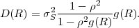 | (6.71) |
By deriving the asymptote for g(R) approaching zero, we obtain the following asymptotic operational distortion rate function for high rates,
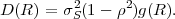 | (6.72) |
The function g(R) represents the operational distortion rate function for scalar quantization of random variables that have unit variance and the same distribution type as the prediction residuals. It should be mentioned that, even at high rates, the distribution of the prediction residuals cannot be derived in a straightforward way, since it is determined by a complicated process that includes linear prediction and quantization. As a rule of thumb based on intuition, at high rates, the reconstructed values S′n are a very close approximation of the original samples Sn and thus the quantization errors Qn = S′n - Sn are very small in comparison to the innovation Zn. Then, we can argue that the prediction residuals Un given by (6.66) are nearly identical to the innovation samples Zn and have thus nearly a Gaussian distribution. Another reason for assuming a Gaussian model is the fact that Gaussian sources are the most difficult to code among all processes with a given autocovariance function. Using a Gaussian model for the prediction residuals, we can replace g(R) in (6.72) by the high rate asymptote for entropy-constrained quantization of Gaussian sources, which yields the following high rate approximation of the operational distortion rate function,
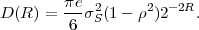 | (6.73) |
Hence, under the intuitive assumption that the distribution of the prediction residuals at high rates is nearly Gaussian, we obtain an asymptotic operational distortion rate function for DPCM quantization of stationary Gauss-Markov processes at high rates that lies 1.53 dB or 0.25 bit per sample above the fundamental rate distortion bound (4.119). The experimental results presented below indicate that our intuitive assumption provides a useful approximation of the operational distortion rate function for DPCM coding of stationary Gauss-Markov processes at high rates.
Even if we use the optimal linear predictor for original sample values inside the DPCM loop, the quantizer design algorithm is not straightforward, since the distribution of the prediction residuals depends on the reconstructed sample values and thus on the quantizer itself.
In order to provide some experimental results for DPCM quantization of Gauss-Markov sources, we use a very simple ECSQ design in combination with a given linear predictor. The vector of prediction parameters hN is given and only the entropy-constrained scalar quantizer is designed. Given a sufficiently large training set {sn}, the quantizer design algorithm can be stated as follows:
The quantizer design algorithm starts with a small value of λ and thus a high rate for which we can assume that reconstruction values are nearly identical to the original sample values. In each iteration of the algorithm, a quantizer is designed for a slightly larger value of λ and thus a slightly lower rate by assuming that the optimal quantizer design does not change significantly. By executing the algorithm, we obtain a sequence of quantizers for different rates. It should however be noted that the quantizer design inside a feedback loop is a complicated problem. We noted that when the value of λ is changed too much from one iteration to the next, the algorithm becomes unstable at low rates. An alternative algorithm for designing predictive quantizers based on conjugate gradient techniques can be found in [8].
For providing experimental results, we considered the stationary Gauss-Markov source with zero mean, unit variance, and a correlation factor of 0.9 that we have used as reference throughout this text. We have run the entropy-constrained Lloyd algorithm for DPCM stated above and measured the prediction error variance σU2, the distortion D, and the entropy of the reconstructed sample values as measure for the transmission rate R. The results of the algorithm are compared to the distortion rate function and to the derived functions for σU2(R) and D(R) for stationary Gauss-Markov sources that are given in (6.70) and (6.71), respectively. For the function g(R) we used the experimentally obtained approximation (5.59) for Gaussian pdfs. It should be noted that the corresponding functional relationships σU2(R) and D(R) are only a rough approximation, since the distribution of the prediction residual Un cannot be assumed to be Gaussian, at least not at low and medium rates.
Fig. 6.8 Linear predictive coding of a stationary Gauss-Markov source with unit variance and a correlation factor of ρ = 0.9. The diagram compares the distortion rate efficiency of ECSQ (without prediction) and ECSQ inside the prediction loop to the (information) distortion rate function D(R). The circles represent experimental data while the solid lines represent derived distortion rate functions. The rate is measured as the entropy of the quantizer output.
In Fig. 6.8, the experimentally obtained data for DPCM coding with entropy-constrained scalar quantization and for entropy-constrained scalar quantization without prediction are compared to the derived operational distortion rate functions using the approximation g(R) for Gaussian sources given in (5.59) and the information rate distortion function. For the shown experimental data and the derived operational distortion rate functions, the rate has been measured as the entropy of the quantizer output. The experimental data clearly indicate that DPCM coding significantly increases the rate distortion efficiency for sources with memory. Furthermore, we note that the derived operational distortion rate functions using the simple approximation for g(R) represent suitable approximations for the experimentally obtained data. At high rates, the measured difference between the experimental data for DPCM and the distortion rate bound is close to 1.53 dB, which corresponds to the space-filling gain of vector quantization as the quantizer dimension approaches infinity. This indicates that DPCM coding of stationary Gauss-Markov sources can fully exploit the dependencies inside the source at high rates and that the derived asymptotic operational distortion rate function (6.73) represents a reasonable approximation for distortion rate efficiency that can be obtained with DPCM coding of stationary Gauss-Markov sources at high rates. At low rates, the distance between the distortion rate bound and the obtained results for DPCM coding increases. A reason is that the variance σU2 of the prediction residuals increases when the rate R is decreased, which is illustrated in Fig. 6.9.
Fig. 6.9 Variance of prediction residual σU2 as function of the bit rate for DPCM coding of a Gauss-Markov source with unit variance and a correlation factor of ρ = 0.9. The circles show the experimental results while the solid line represents the derived approximation. The rate is measured as the entropy of the quantizer output.
The DPCM gain can be defined as the ratio of the operational distortion rate functions for scalar quantization and DPCM coding,
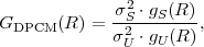 | (6.74) |
where gS(R) and gU(R) represent the normalized operational distortion rate functions for scalar quantization of the source signal and the prediction residuals, respectively. At high rates and under our intuitive assumption that the prediction residuals are nearly Gaussian, the normalized operational distortion rate function gU(R) for scalar quantization of the prediction residuals becomes equal to the normalized operational distortion rate function gS(R) for scalar quantization of the original samples. Then, the asymptotic coding gain for DPCM coding of stationary Gauss-Markov sources at high rates is approximately
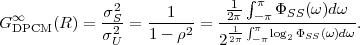 | (6.75) |
6.4.2 Adaptive Differential Pulse Code Modulation
So far we have discussed linear prediction and DPCM coding for stationary sources. However, the input signals in practical coding systems are usually not stationary and thus a fixed predictor is not well suited. For nonstationary signals the predictor needs to be adapted based on local signal characteristics. The adaptation method is either signaled from the sender to the receiver (forward adaptation) by side information or simultaneously derived at both sides using a prescribed algorithm (backward adaptation).
A block diagram for a predictive codec with forward adaptation is shown in Fig. 6.10. The encoder sends new prediction coefficients to the decoder, which produces additional bit rate. It is important to balance the increased bit rate for the adaptation signal against the bit rate reduction resulting from improved prediction. In practical codecs, the adaptation signal is send infrequently at well-defined intervals. A typical choice in image and video coding is to adapt the predictor on a block-by-block basis.
A block diagram for a predictive codec with backward adaptation is shown in Fig. 6.11. The prediction signal is derived from the previously decoded signal. It is advantageous relative to forward adaptation in that no additional bit rate is needed to signal the modifications of the predictor. Furthermore, backward adaptation does not introduced any additional encoding-decoding delay. The accuracy of the predictor is governed by the statistical properties of the source signal and the used adaptation algorithm. A drawback of backward adaptation is that the simultaneous computation of the adaptation signal is its increased sensitivity to transmission errors.
6.5 Summary of Predictive Coding
In this chapter, we have discussed predictive coding. We introduced the concept of prediction as a procedure of estimating the value of a random variable based on already observed random variables. If the efficiency of a predictor is measured by the mean squared prediction error, the optimal prediction value is given by the conditional expectation of the random variable to be predicted given the observed random variables. For particular important sources such as Gaussian sources and autoregressive (AR) processes, the optimal predictor represents an affine function of the observation vector. A method to generally reduce the complexity of prediction is to constrain its structure to linear or affine prediction. The difference between linear and affine prediction is that the additional constant offset in affine prediction can compensate for the mean of the input signal.
For stationary random processes, the optimal linear predictor is given by the solution of the Yule-Walker equations and depends only on the autocovariances of the source signal. If an optimal affine predictor is used, the resulting prediction residual is orthogonal to each of the observed random variables. The optimal linear predictor for a stationary AR(m) process has m prediction coefficients, which are equal to the model parameters of the input process. A stationary Gauss-Markov process is a stationary AR(1) process and hence the optimal linear predictor has a single prediction coefficient, which is equal to the correlation coefficient of the Gauss-Markov process. It is important to note that a non-matched predictor can increase the prediction error variance relative to the signal variance.
Differential pulse code modulation (DPCM) is the dominant structure for the combination of prediction and scalar quantization. In DPCM, the prediction is based on quantized samples. The combination of DPCM and entropy-constrained scalar quantization (ECSQ) has been analyzed in great detail for the special case of stationary Gauss-Markov processes. It has been shown that the prediction error variance is dependent on the bit rate. The derived approximation for high rates, which has been verified by experimental data, indicated that for stationary Gauss-Markov sources the combination of DPCM and ECSQ achieves the shape and memory gain of vector quantization at high rates.
This is the html version of the book:
Thomas Wiegand and Heiko Schwarz (2010): "Source Coding: Part I of Fundamentals of Source and Video Coding", Now Publishers, Foundations and Trends® in Signal Processing: Vol. 4: No 1-2, pp 1-222. (pdf version of the book)
7 Transform Coding
Similar to predictive coding, which we reviewed in the last chapter, transform coding is a concept for exploiting statistically dependencies of a source at a low complexity level. Transform coding is used in virtually all lossy image and video coding applications.
The basic structure of a typical transform coding system is shown in Fig. 7.1. A vector of a fixed number N input samples s is converted into a vector of N transform coefficients u using an analysis transform A. The transform coefficients ui, with 0 ≤ i < N, are quantized independently of each other using a set of scalar quantizers. The vector of N reconstructed samples s′ is obtained by transforming the vector of reconstructed transform coefficients u′ using a synthesis transform B.
In all practically used video coding systems, the analysis and synthesis transforms A and B are orthogonal block transforms. The sequence of source samples {sn} is partitioned into vectors s of adjacent samples and the transform coding consisting of an orthogonal analysis transform, scalar quantization of the transform coefficients, and an orthogonal synthesis transform is independently applied to each vector of samples. Since finally a vector s of sources samples is mapped to a vector s′ of reconstructed samples, transform coding systems form a particular class of vector quantizers. The benefit in comparison to unconstrained vector quantization is that the imposed structural constraint allows implementations at a significantly lower complexity level.
The typical motivation for transform coding is the decorrelation and energy concentration effect. Transforms are designed in a way that, for typical input signals, the transform coefficients are much less correlated than the original source samples and the signal energy is concentrated in a few transform coefficients. As a result, the obtained transform coefficients have a different importance and simple scalar quantization becomes more effective in the transform domain than in the original signal space. Due to this effect, the memory advantage of vector quantization can be exploited to a large extend for typical source signals. Furthermore, by using entropy-constrained quantization for the transform coefficients also the shape advantage can be obtained. In comparison to unconstrained vector quantization, the rate distortion efficiency is basically reduced by the space-filling advantage, which can only be obtained by a significant increase in complexity.
For image and video coding applications, another advantage of transform coding is that the quantization in the transform domain often leads to an improvement of the subjective quality relative to a direct quantization of the source samples with the same distortion, in particular for low rates. The reason is that the transform coefficients contain information with different importance for the viewer and can therefore be treated differently. All perceptual distortion measures that are known to provide reasonable results weight the distortion in the transform domain. The quantization of the transform coefficients can also be designed in a way that perceptual criteria are taken into account.
In contrast to video coding, the transforms that are used in still image coding are not restricted to the class of orthogonal block transforms. Instead, transforms that do not process the input signal on a block-by-block basis have been extensively studied and included into recent image coding standards. One of these transforms is the so-called discrete wavelet transform, which decomposes an image into components that correspond to band-pass filtered and downsampled versions of the image. Discrete wavelet transforms can be efficiently implemented using cascaded filter banks. Transform coding that is based on a discrete wavelet transform is also referred to as subband coding and is for example used in the JPEG 2000 standard [41, 72]. Another class of transforms are the lapped block transforms, which are basically applied on a block-by-block basis, but are characterized by basis functions that overlap the block boundaries. As a result, the transform coefficients for a block do not only depend on the samples inside the block, but also on samples of neighboring blocks. The vector of reconstructed samples for a block is obtained by transforming a vector that includes the transform coefficients of the block and of neighboring blocks. A hierarchical lapped transform with biorthogonal basis functions is included in the latest image coding standard JPEG XR [42]. The typical motivation for using wavelet transforms or lapped block transforms in image coding is that the nature of these transforms avoids the blocking artifacts which are obtained by transform coding with block-based transforms at low bit rates and are considered as one of the most disturbing coding artifacts. In video coding, wavelet transforms and lapped block transforms are rarely used due to the difficulties in efficiently combining these transforms with inter-picture prediction techniques.
In this chapter, we discuss transform coding with orthogonal block transforms, since this is the predominant transform coding structure in video coding. For further information on transform coding in general, the reader is referred to the tutorials [20] and [10]. An introduction to wavelet transforms and subband coding is given in the tutorials [74, 76] and [77]. As a reference for lapped blocks transforms and their application in image coding we recommend [62] and [53].
7.1 Structure of Transform Coding Systems
The basic structure of transform coding systems with block transforms is shown in Fig. 7.1. If we split the scalar quantizers Qk, with k = 0,…,N - 1, into an encoder mapping αk that converts the transform coefficients into quantization indexes and a decoder mapping βk that converts the quantization indexes into reconstructed transform coefficients and additionally introduce a lossless coding γ for the quantization indexes, we can decompose the transform coding system shown in Fig. 7.1 into a transform encoder and a transform decoder as illustrated in Fig. 7.2.
In the transform encoder, the analysis transform converts a vector
s = (s0, ,sN-1)T of N source samples into a vector of N transform
coefficients u = (u0,
,sN-1)T of N source samples into a vector of N transform
coefficients u = (u0, ,uN-1)T . Each transform coefficient uk is then
mapped onto a quantization index ik using an encoder mapping αk. The
quantization indexes of all transform coefficients are coded using a lossless
mapping γ, resulting in a sequence of codewords b.
,uN-1)T . Each transform coefficient uk is then
mapped onto a quantization index ik using an encoder mapping αk. The
quantization indexes of all transform coefficients are coded using a lossless
mapping γ, resulting in a sequence of codewords b.
In the transform decoder, the sequence of codewords b is mapped to the
set of quantization indexes ik using the inverse lossless mapping γ-1.
The decoder mappings βk convert the quantization indexes ik into
reconstructed transform coefficients u′k. The vector of N reconstructed
samples s′ = (s′0, ,s′N-1)T is obtained by transforming the vector of N
reconstructed transform coefficients u′ = (u′0,
,s′N-1)T is obtained by transforming the vector of N
reconstructed transform coefficients u′ = (u′0, ,u′N-1)T using the
synthesis transform.
,u′N-1)T using the
synthesis transform.
7.2 Orthogonal Block Transforms
In the following discussion of transform coding, we restrict our considerations to stationary sources and transform coding systems with the following properties:
For linear block transforms of size N, each component of an N-dimensional output vector represents a linear combination of the components of the N-dimensional input vector. A linear block transform can be written as a matrix multiplication. The analysis transform, which maps a vector of source samples s to a vector of transform coefficients u, is given by
 | (7.1) |
where the matrix A is referred to as the analysis transform matrix. Similarly, the synthesis transform, which maps a vector of reconstructed transform coefficients u′ to a vector of reconstructed samples s′, can be written as
 | (7.2) |
where the matrix B represents the synthesis transform matrix.
The perfect reconstruction property specifies that the synthesis transform matrix is the inverse of the analysis transform matrix, B = A-1. If the transform coefficients are not quantized, i.e., if u′ = u, the vector of reconstructed samples is equal to the vector of source samples,
 | (7.3) |
If an invertible analysis transform A produces independent transform coefficients and the component quantizers reconstruct the centroids of the quantization intervals, the inverse of the analysis transform is the optimal synthesis transform in the sense that it yields the minimum distortion among all linear transforms given the coded transform coefficients. It should, however, be noted that if these conditions are not fulfilled, a synthesis transform B that is not equal to the inverse of the analysis transform may reduce the distortion [20].
An analysis transform matrix A forms an orthonormal basis if its basis vectors given by the rows of the matrix are orthogonal to each other and have the length 1. Matrices with this property are referred to as unitary matrices. The corresponding transform is said to be an orthogonal transform. The inverse of a unitary matrix A is its conjugate transpose, A-1 = A†. A unitary matrix with real entries is called an orthogonal matrix and its inverse is equal to its transpose, A-1 = AT . For linear transform coding systems with the perfect reconstruction property and orthogonal matrices, the synthesis transform is given by
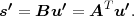 | (7.4) |
Unitary transform matrices are often desirable, because the mean square error between a reconstruction and source vector can be minimized with independent scalar quantization of the transform coefficients. Furthermore, as we will show below, the distortion in the transform domain is equal to the distortion in the original signal space. In practical transform coding systems, it is usually sufficient to require that the basis vectors are orthogonal to each other. The different norms can be easily taken into account in the quantizer design.
We can consider a linear analysis transform A as optimal if the transform coding system consisting of the analysis transform A, optimal entropy-constrained scalar quantizers for the transform coefficients (which depend on the analysis transform), and the synthesis transform B = A-1 yields a distortion for a particular given rate that is not greater than the distortion that would be obtained with any other transform at the same rate. In this respect, a unitary transform is optimal for the MSE distortion measure if it produces independent transform coefficients. Such a transform does, however, not exist for all sources. Depending on the source signal, a non-unitary transform may be superior [20, 13].
An important property of transform coding systems with the perfect reconstruction property and unitary transforms is that the MSE distortion is preserved in the transform domain. For the general case of complex transform matrices, the MSE distortion between the reconstructed samples and the source samples can be written as
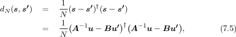
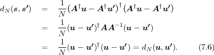
Another important property for orthogonal transforms can be derived by considering the autocovariance matrix for the random vectors U of transform coefficients,
 | (7.7) |
With U = AS and A-1 = AT , we obtain
 | (7.8) |
where CSS denotes the autocovariance matrix for the random vectors S of original source samples. It is known from linear algebra that the trace tr(X) of a matrix X is similarity-invariant,
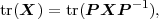 | (7.9) |
with P being an arbitrary invertible matrix. Since the trace of an autocovariance matrix is the sum of the variances of the vector components, the arithmetic mean of the variances σi2 of the transform coefficients is equal to the variance σS2 of the original samples,
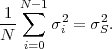 | (7.10) |
An interpretation of the matrix multiplication in (7.2) is that the vector of reconstructed samples s′ is represented as a linear combination of the columns of the synthesis transform matrix B, which are also referred to as the basis vectors bk of the synthesis transform. The weights in this linear combination are given by the reconstructed transform coefficients u′k and we can write
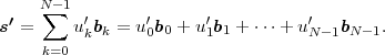 | (7.11) |
Similarly, the original signal vector s is represented by a linear combination of the basis vectors ak of the inverse analysis transform, given by the columns of A-1,
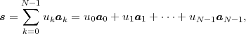 | (7.12) |
where the weighting factors are the transform coefficients uk. If the analysis transform matrix is orthogonal (A-1 = AT ), the columns of A-1 are equal to the rows of A. Furthermore, the basis vectors ak are orthogonal to each other and build a coordinate system with perpendicular axes. Hence, there is a unique way to represent a signal vector s in the new coordinate system given by the set of basis vectors {ak}. Each transform coefficient uk is given by the projection of the signal vector s onto the corresponding basis vector ak, which can be written as scalar product
 | (7.13) |
Since the coordinate system spanned by the basis vectors has perpendicular axes and the origin coincides with the origin of the signal coordinate system, an orthogonal transform specifies rotations and reflections in the N-dimensional Euclidean space. If the perfect reconstruction property (B = A-1) is fulfilled, the basis vectors bk of the synthesis transform are equal to the basis vectors ak of the analysis transform and the synthesis transform specifies the inverse rotations and reflections of the analysis transform.
As a simple example, we consider the following orthogonal 2 × 2 synthesis matrix,
![[ ]
[ -1-- 1 1
B = b0b1] = √ 2 1 - 1 .](VBpart1676x.png) | (7.14) |
The analysis transform matrix A is given by the transpose of the synthesis matrix, A = BT . The transform coefficients uk for a given signal vector s are the scalar products of the signal vector s and the basis vectors bk. For a signal vector s=[4,3]T , we obtain
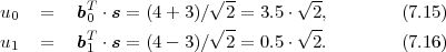
![s = u0 ⋅b0 + u1 ⋅b1
[ 4 ] √ -- 1 [ 1 ] √ -- 1 [ 1 ]
= (3.5⋅ 2)⋅ √-- (0.5⋅ 2)⋅ √-- . (7.17)
3 2 1 2 - 1](VBpart1678x.png)
Fig. 7.4 illustrates the effect of a decorrelating orthogonal transform on the example of the given 2 × 2 transform for stationary zero-mean Gauss-Markov sources with unit variance and different correlation coefficients ρ. If the source samples are not correlated (ρ = 0), the transform does not have any effect. But for correlated sources, the transform rotates the distribution of the source vectors in a way that the primary axes of the distribution are aligned with axes of the coordinate system in the transform domain. For the example 2 × 2 transform this has the effect that the variance for one transform coefficient is minimized while the variance of the other transform coefficient is maximized. The signal energy is shifted toward the first transform coefficient U0.
Fig. 7.4 Effect of a decorrelating orthogonal transform on the example of the 2 × 2 transform given in (7.14) for stationary Gauss-Markov sources with zero mean, unit variance and different correlation coefficients ρ: (top) distribution of sources vectors; (bottom) distribution of transform coefficient vectors.
In Fig. 7.5 the quantization cells for scalar quantization in the original signal space are compared with the quantization cells for transform coding. As discussed in Chapter 5, the effective quantization cells for simple scalar quantization in the N-dimensional signal space are hyperrectangles that are aligned with the axes of the coordinate system as illustrated in the left diagram of Fig. 7.5. For transform coding, the quantization cells in the transform domain are hyperrectangles that are aligned with the axes of the coordinate system of the transform coefficients (middle diagram of Fig. 7.5). In the original signal space, the quantization cells are still hyperrectangles, but the grid of quantization cells is rotated and aligned with the basis vectors of the orthogonal transform as shown in the right diagram of Fig. 7.5. As a rough approximation, the required bit rate can be considered as proportional to the number of quantization cells associated with appreciable probabilities in the coordinate directions of the quantization grid. This indicates that, for correlated sources, transform coding yields a higher rate distortion efficiency than scalar quantization in the original domain.
Fig. 7.5 Comparison of transform coding and scalar quantization in the original signal space: (left) source distribution and quantization cells for scalar quantization; (middle) distribution of transform coefficients and quantization cells in the transform domain; (right) source distribution and quantization cells for transform coding in the original signal space.
7.3 Bit Allocation for Transform Coefficients
Before we discuss decorrelating transforms in more detail, we analyze the problem of bit allocation for transform coefficients. As mentioned above, the transform coefficients have usually a different importance and hence the overall rate distortion efficiency of a transform coding system depends on a suitable distribution of the overall rate R among the transform coefficients. A bit allocation is optimal if a given overall rate R is distributed in a way that the resulting overall distortion D is minimized. If we use the MSE distortion measure, the distortion in the original signal space is equal to the distortion in the transform domain. Hence, with Ri representing the component rates for the transform coefficients ui and Di(Ri) being the operational distortion rate functions for the component quantizers, we want to minimize
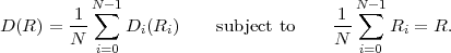 | (7.18) |
As has been discussed in sec. 5.2.2, the constrained optimization problem (7.18) can be reformulated as an unconstrained minimization of the Lagrangian cost functional J = D + λR. If we assume that the operational distortion rate functions Di(Ri) for the component quantizers are convex, the optimal rate allocation can be found by setting the partial derivatives of the Lagrangian functional J with respect to the component rates Ri equal to 0,
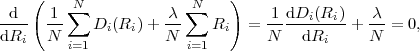 | (7.19) |
which yields
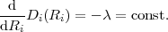 | (7.20) |
This so-called Pareto condition states that, for optimal bit allocation, all component quantizers should be operated at equal slopes of their operational distortion rate functions Di(Ri).
In sec. 5.2.4, we have shown that the operational distortion rate function of scalar quantizers can be written as
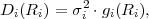 | (7.21) |
where σi2 is the variance of the input source and gi(Ri) is the operational distortion rate function for the normalized distribution with unit variance. In general, it is justified to assume that gi(Ri) is a non-negative, strictly convex function and has a continuous first derivative g′i(Ri) with g′i(∞) = 0. Then, the Pareto condition yields
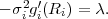 | (7.22) |
As discussed in sec. 4.4, it has to be taken into account that the component rate Ri for a particular transform coefficient cannot be negative. If λ ≥-σi2g′i(0), the quantizer for the transform coefficient ui cannot be operated at the given slope λ. In this case, it is optimal to set the component rate Ri equal to zero. The overall distortion is minimized if the overall rate is spent for coding only the transform coefficients with -σi2g′i(0) > λ. This yields the following bit allocation rule,
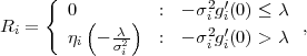 | (7.23) |
where ηi(⋅) denotes the inverse of the derivative g′i(⋅). Since g′i(Ri) is a continuous strictly increasing function for Ri ≥ 0 with g′i(∞) = 0, the inverse ηi(x) is a continuous strictly increasing function for the range g′i(0) ≤ x ≤ 0 with ηi(f′i(0)) = 0 and ηi(0) = ∞.
7.3.1 Approximation for Gaussian Sources
If the input signal has a Gaussian distribution, the distributions for all transform coefficients are also Gaussian, since the signal for each transform coefficient represents a linear combination of Gaussian sources. Hence, we can assume that the operational distortion rate function for all component quantizers is given by
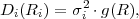 | (7.24) |
where g(R) represents the operational distortion rate function for Gaussian sources with unit variance. In order to derive an approximate formula for the optimal bit allocation, we assume that the component quantizers are entropy-constrained scalar quantizers and use the approximation (5.59) for g(R) that has been experimentally found for entropy-constrained scalar quantization of Gaussian sources in sec. 5.2.4,
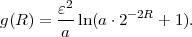 | (7.25) |
The factor ε2 is equal to πe∕6 and the model parameter a is approximately 0.9519. The derivative g′(R) and its inverse η(x) are given by
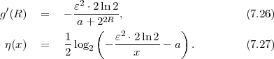
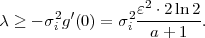 | (7.28) |
With the parameter
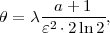 | (7.29) |
we obtain the bit allocation rule
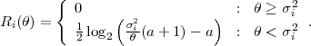 | (7.30) |
The resulting component distortions are given by
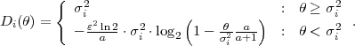 | (7.31) |
If the variances σi2 of the transform coefficients are known, the approximation of the operational distortion rate function for transform coding of Gaussian sources with entropy-constrained scalar quantization is given by the parametric formulation
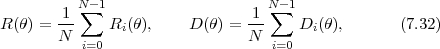
In the following, we assume that the overall rate R is high enough so that all component quantizers are operated at high component rates Ri. In sec. 5.2.3, we have shown that the asymptotic operational distortion rate functions for scalar quantizers can be written as
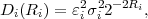 | (7.33) |
where the factor εi2 depends only on the type of the source distribution and the used scalar quantizer. Using these high rate approximations for the component quantizers, the Pareto condition becomes
 | (7.34) |
At high rates, an optimal bit allocation is obtained if all component distortions Di are the same. Setting the component distortions Di equal to the overall distortion D, yields
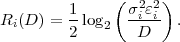 | (7.35) |
For the overall operational rate distortion function, we obtain
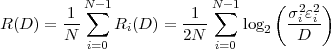 | (7.36) |
With the geometric means of the variances σi2 and the factors ϵi2,
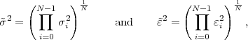 | (7.37) |
the asymptotic operational distortion rate function for high rates can be written as
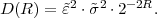 | (7.38) |
It should be noted that this result can also be derived without using the Pareto condition, which was obtained by calculus. Instead, we can use the inequality of arithmetic and geometric means and derive the high rate approximation similar to the rate distortion function for Gaussian sources with memory in sec. 4.4.
For Gaussian sources, all transform coefficients have a Gaussian distribution (see sec. 7.3.1), and thus all factors εi2 are the same. If entropy-constrained scalar quantizers are used, the factors εi2 are equal to πe∕6 (see sec. 5.2.3) and the asymptotic operational distortion rate function for high rates is given by
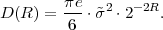 | (7.39) |
The effectiveness of a transform is often specified by the transform coding gain, which is defined as the ratio of the operational distortion rate functions for scalar quantization and transform coding. At high rates, the transform coding gain is given by
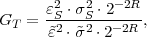 | (7.40) |
where εS2 is the factor of the high rate approximation of the operational distortion rate function for scalar quantization in the original signal space and σS2 is the variance of the input signal.
By using the relationship (7.10), the high rate transform gain for Gaussian sources can be expressed as the ratio of the arithmetic and geometric mean of the transform coefficient variances,
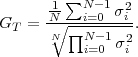 | (7.41) |
The high rate transform gain for Gaussian sources is maximized if the geometric mean is minimized. The transform that minimizes the geometric mean is the Karhunen Loève Transform, which will be discussed in the next section.
7.4 The Karhunen Loève Transform (KLT)
Due to its importance in the theoretical analysis of transform coding we discuss the Karhunen Loève Transform (KLT) in some detail in the following. The KLT is an orthogonal transform that decorrelates the vectors of input samples. The transform matrix A is dependent on the statistics of the input signal.
Let S represent the random vectors of original samples of a stationary input sources. The random vectors of transform coefficients are given by U = AS and for the autocorrelation matrix of the transform coefficients we obtain
 | (7.42) |
where
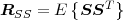 | (7.43) |
denotes the autocorrelation matrix of the input process. To get uncorrelated transform coefficients, the orthogonal transform matrix A has to be chosen in a way that the autocorrelation matrix RUU becomes a diagonal matrix. Equation (7.42) can be slightly reformulated as
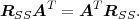 | (7.44) |
With bi representing the basis vectors of the synthesis transform, i.e., the column vectors of A-1 = AT and the row vectors of A, it becomes obvious that RUU is a diagonal matrix if the eigenvector equation
 | (7.45) |
is fulfilled for all basis vectors bi. The eigenvalues ξi represents the elements rii on the main diagonal of the diagonal matrix RUU. The rows of the transform matrix A are build by a set of unit-norm eigenvectors of RSS that are orthogonal to each other. The autocorrelation matrix for the transform coefficients RUU is a diagonal matrix with the eigenvalues of RSS on its main diagonal. The transform coefficient variances σi2 are equal to the eigenvalues ξi of the autocorrelation matrix RSS.
A KLT exists for all sources, since symmetric matrices as the autocorrelation matrix RSS are always orthogonally diagonizable. There exist more than one KLT of any particular size N > 1 for all stationary sources, because the rows of A can be multiplied by -1 or permuted without influencing the orthogonality of A or the diagonal form of RUU. If the eigenvalues of RSS are not distinct, there are additional degrees of freedom for constructing KLT transform matrices. Numerical methods for calculating the eigendecomposition RSS = AT diag(ξi)A of real symmetric matrices RSS are the classical and the cyclic Jacobi algorithm [43, 18].
For nonstationary sources, transform coding with a single KLT transform matrix is suboptimal. Similar to the predictor in predictive coding, the transform matrix should be adapted based on the local signal statistics. The adaptation can be realized either as forward adaptation or as backward adaptation. With forward adaptive techniques, the transform matrix is estimated at the encoder and an adaptation signal is transmitted as side information, which increases the overall bit rate and usually introduces an additional delay. In backward adaptive schemes, the transform matrix is simultaneously estimated at the encoder and decoder side based on already coded samples. Forward adaptive transform coding is discussed in [12] and transform coding with backward adaptation is investigated in [21].
7.4.1 On the Optimality of the KLT
We showed that the KLT is an orthogonal transform that yields decorrelated transform coefficients. In the following, we show that the KLT is also the orthogonal transform that maximizes the rate distortion efficiency for stationary zero-mean Gaussian sources if optimal scalar quantizers are used for quantizing the transform coefficients. The following proof was first delineated in [19].
We consider a transform coding system with an orthogonal N ×N analysis transform matrix A, the synthesis transform matrix B = AT , and scalar quantization of the transform coefficients. We further assume that we use a set of scalar quantizers that are given by scaled versions of a quantizer for unit variance for which the operational distortion rate function is given by a nonincreasing function g(R). The decision thresholds and reconstruction levels of the quantizers are scaled according to the variances of the transform coefficients. Then, the operational distortion rate function for each component quantizer is given by
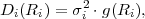 | (7.46) |
where σi2 denotes the variance of the corresponding transform coefficient (cp. sec. 5.2.4). It should be noted that such a setup is optimal for Gaussian sources if the function g(R) is the operational distortion rate function of an optimal scalar quantizer. The optimality of a quantizer may depend on the application. As an example, we could consider entropy-constrained Lloyd quantizers as optimal if we assume a lossless coding that achieves an average codeword length close to the entropy. For Gaussian sources, the transform coefficients have also a Gaussian distribution. The corresponding optimal component quantizers are scaled versions of the optimal quantizer for unit variance and their operational distortion rate functions are given by (7.46).
We consider an arbitrary orthogonal transform matrix A0 and an
arbitrary bit allocation given by the vector b = (R0, RN-1)T
with ∑
i=0N-1Ri = R. Starting with the given transform matrix
A0 we apply an iterative algorithm that generates a sequence of
orthonormal transform matrices {Ak}. The corresponding autocorrelation
matrices are given by R(Ak) = AkRSSAkT with RSS denoting the
autocorrelation matrix of the source signal. The transform coefficient
variances σi2(Ak) are the elements on the main diagonal of R(Ak) and the
distortion rate function for the transform coding system is given
by
RN-1)T
with ∑
i=0N-1Ri = R. Starting with the given transform matrix
A0 we apply an iterative algorithm that generates a sequence of
orthonormal transform matrices {Ak}. The corresponding autocorrelation
matrices are given by R(Ak) = AkRSSAkT with RSS denoting the
autocorrelation matrix of the source signal. The transform coefficient
variances σi2(Ak) are the elements on the main diagonal of R(Ak) and the
distortion rate function for the transform coding system is given
by
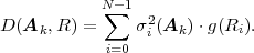 | (7.47) |
Each iteration Ak Ak+1 shall consists of the following two steps:
Itis obvious that the reordering step does not increase the distortion, i.e., D(PkAk,R) ≤ D(Ak,R). Furthermore, for each pair of variances σi2(PkAk) ≥ σj2(PkAk), it implies g(Ri) ≤ g(Rj); otherwise, the distortion D(PkAk,R) could be decreased by switching the i-th and j-th row of the matrix PkAk. A Jacobi rotation that zeros the element rij of the autocorrelation matrix R(PkAk) in R(Ak+1) does only change the variances for the i-th and j-th transform coefficient. If σi2(PkAk) ≥ σj2(PkAk), the variances are modified according to
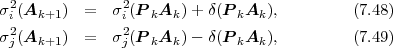
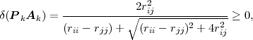 | (7.50) |
and rij being the elements of the matrix R(PkAk). The overall distortion for the transform matrix Ak+1 will never become smaller than the overall distortion for the transform matrix Ak,
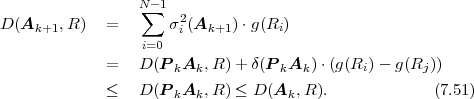
We have shown that the KLT is the orthogonal transform that minimizes the distortion for a set of scalar quantizers that represent scaled versions of a given quantizer for unit variance. In particular, the KLT is the optimal transform for Gaussian sources if optimal scalar quantizers are used [19]. The KLT produces decorrelated transform coefficients. However, decorrelation does not necessarily imply independence. For non-Gaussian sources, other orthogonal transforms or nonorthogonal transforms can be superior with respect to the coding efficiency [20, 13].
As an example, we consider the 3 ×3 KLT for a stationary Gauss-Markov process with zero mean, unit variance, and a correlation coefficient of ρ = 0.9. We assume a bit allocation vector b = [5,3,2] and consider entropy-constrained scalar quantizers. We further assume that the high-rate approximation of the operational distortion rate function Di(Ri) = ε2σi22-2Ri with ε2 = πe∕6 is valid for the considered rates. The initial transform matrix A0 shall be the matrix of the DCT-II transform, which we will later introduce in sec. 7.5.3. The autocorrelation matrix RSS and the initial transform matrix A0 are given by
![[ ] [ ]
1 0.9 0.81 0.5774 0.5774 0.5774
Rs = 0.9 1 0.9 , A0 = 0.7071 0 - 0.7071 .
0.81 0.9 1 0.4082 -0.8165 0.4082](VBpart1732x.png) | (7.52) |
For the transform coefficients, we obtain the autocorrelation matrix
![[ ]
2.74 0 - 0.0424
R (A0) = 0 0.19 0 .
-0.0424 0 0.07](VBpart1733x.png) | (7.53) |
The distortion D(A0,R) for the initial transform is equal to 0.01426. We now investigate the effect of the first iteration of the algorithm described above. For the given relative ordering in the bit allocation vector b, the optimal reordering matrix P0 is the identity matrix. The Jacobi rotation matrix Q0 and the resulting new transform matrix A1 are given by
![[ ] [ ]
0.9999 0 - 0.0159 0.5708 0.5902 0.5708
Q0 = 0 1 0 , A1 = 0.7071 0 -0.7071 .
0.0159 0 0.9999 0.4174 -0.8072 0.4174](VBpart1734x.png) | (7.54) |
The parameter δ(P0A0) is equal to 0.000674. The distortion D(A1,R) is equal to 0.01420. In comparison to the distortion for the initial transform matrix A0, it has been reduced by about 0.018 dB. The autocorrelation matrix R(A1) for the new transform coefficients is given by
![[ 2.7407 0 0 ]
R (A1 ) = 0 0.19 0 .
0 0 0.0693](VBpart1735x.png) | (7.55) |
The autocorrelation matrix has already become a diagonal matrix after the first iteration. The transform given by A1 represents a KLT for the given source signal.
7.4.2 Asymptotic Operational Distortion Rate Function
In sec. 7.3.2, we considered the bit allocation for transform coding at high rates. An optimal bit allocation results in constant component distortions Di, which are equal to the overall distortion D. By using the high rate approximation Di(Ri) = εi2σi22-2Ri for the operational distortion rate function of the component quantizers, we derived the overall operational distortion rate function given in (7.36). For Gaussian sources and entropy-constrained scalar quantization, all parameters εi2 are equal to ε = πe∕6. And if we use a KLT of size N as transform matrix, the transform coefficient variances σi2 are equal to the eigenvalues ξi(N) of the N-th order autocorrelation matrix RN for the input process. Hence, for Gaussian sources and a transform coding system that consists of a KLT of size N and entropy-constrained scalar quantizers for the transform coefficients, the high rate approximation for the overall distortion rate function can be written as
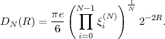 | (7.56) |
The larger we choose the transform size N of the KLT, the more the samples of the input source are decorrelated. For deriving a bound for the operational distortion rate function at high rates, we consider the limit for N approaching infinity. By applying Grenander and Szegö’s theorem (4.76) for sequences of Toeplitz matrices, the limit of (7.56) for N approaching infinity can be reformulated using the power spectral density ΦSS(ω) of the input source. For Gaussian sources, the asymptotic operational distortion rate function for high rates and large transform dimensions is given by
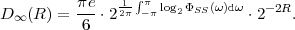 | (7.57) |
A comparison with the Shannon lower bound (4.77) for zero-mean Gaussian sources shows that the asymptotic operational distortion rate function lies 1.53 dB or 0.25 bit per sample above this fundamental bound. The difference is equal to the space-filling advantage of high-dimensional vector quantization. For zero-mean Gaussian sources and high rates, the memory and shape advantage of vector quantization can be completely exploited using a high-dimensional transform coding.
By using the relationship σS2 =  ∫
-ππΦSS(ω)dω for the variance of
the input source, the asymptotic transform coding gain for zero-mean
Gaussian sources can be expressed as the ratio of the arithmetic and
geometric means of the power spectral density,
∫
-ππΦSS(ω)dω for the variance of
the input source, the asymptotic transform coding gain for zero-mean
Gaussian sources can be expressed as the ratio of the arithmetic and
geometric means of the power spectral density,
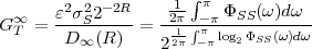 | (7.58) |
The asymptotic transform coding gain at high rates is identical to the approximation for the DPCM coding gain at high rates (6.75).
We now consider the special case of zero-mean Gauss-Markov sources. The product of the eigenvalues ξi(N) of a matrix RN is always equal to the determinant |RN| of the matrix. And for zero-mean sources, the N-th order autocorrelation matrix RN is equal to the N-th order autocovariance matrix CN. Hence, we can replace the product of the eigenvalues in (7.56) with the determinant |CN| of the N-th order autocovariance matrix. Furthermore, for Gauss-Markov sources, the determinant of the N-th order autocovariance matrix can be expressed according to (2.50). Using these relationships, the operational distortion rate function for zero-mean Gauss-Markov sources and a transform coding system with an N-dimensional KLT and entropy-constrained component quantizers is given by
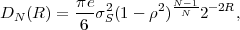 | (7.59) |
where σS2 and ρ denote the variance and the correlation coefficient of the input source. For the corresponding transform gain, we obtain
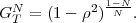 | (7.60) |
The asymptotic operational distortion rate function and the asymptotic transform gain for high rates and N approaching infinity are given by
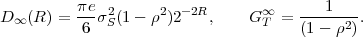 | (7.61) |
7.4.3 Performance for Gauss-Markov Sources
Fig. 7.6 Transform coding of a Gauss-Markov source with zero mean, unit variance, and a correlation coefficient of ρ = 0.9. The diagram compares the efficiency of direct ECSQ and transform coding with ECSQ to the distortion rate function D(R). The circles represent experimental data while the solid lines represent calculated curves. The rate is measured as the average of the entropies for the outputs of the component quantizers.
For demonstrating the effectiveness of transform coding for correlated input sources, we used a Gauss-Markov source with zero mean, unit variance, and a correlation coefficient of ρ = 0.9 and compared the rate distortion efficiency of transform coding with KLT’s of different sizes N and entropy-constrained scalar quantization (ECSQ) with the fundamental rate distortion bound and the rate distortion efficiency for ECSQ of the input samples. The experimentally obtained data and the calculated distortion rate curves are shown in Fig. 7.6. The rate was determined as average of the entropies of the quantizer outputs. It can be seen that transform coding significantly increases the coding efficiency relative to direct ECSQ. An interesting fact is that for transform sizes larger than N = 4 the distance to the fundamental rate distortion bound at low rates is less than at high rates. A larger transform size N generally yields a higher coding efficiency. However, the asymptotic bound (7.61) is already nearly achieved for a moderate transform size of N = 16 samples. A further increase of the transform size N would only slightly improve the coding efficiency for the example source. This is further illustrated in Fig. 7.7, which shows the transform coding gain as function of the transform size N.
Fig. 7.7 Transform gain as function of the transform size N for a zero-mean Gauss-Markov source with a correlation factor of ρ = 0.9.
7.5 Signal-Independent Unitary Transforms
Although the KLT has several desirable properties, it is not used in practically video coding applications. One of the reasons is that there are no fast algorithms for calculating the transform coefficients for a general KLT. Furthermore, since the KLT is signal-dependent, a single transform matrix is not suitable for all video sequences, and adaptive schemes are only implementable at an additional computational complexity. In the following, we consider signal-independent transforms. The transform that is used in all practically used video coding schemes is the discrete cosine transform (DCT), which will be discussed in sec. 7.5.3. In addition, we will briefly review the Walsh-Hadamard transform and, for motivating the DCT, the discrete Fourier transform.
7.5.1 The Walsh-Hadamard Transform (WHT)
The Walsh-Hadamard transform is a very simple orthogonal transform that can be implemented using only additions and a final scaling. For transform sizes N that represent positive integer power of 2, the transform matrix AN is recursively defined by
![[ ]
√1-- AN ∕2 AN ∕2
AN = 2 AN ∕2 - AN ∕2 with A1 = [1].](VBpart1747x.png) | (7.62) |
When ignoring the constant normalization factor, the Hadamard transform matrices only consist of entries equal to 1 and -1 and, hence, the transform coefficients can be calculated very efficiently. However, due to its piecewise-constant basis vectors, the Hadamard transform produces subjectively disturbing artifacts if it is combined with strong quantization of the transform coefficients. In video coding, the Hadamard transform is only used for some special purposes. An example is the second-level transform for chroma coefficients in H.264/AVC [36]
7.5.2 The Discrete Fourier Transform (DFT)
One of the most important transforms in communications engineering and signal processing is the Fourier transform. For discrete-time signals of a finite length N, the discrete Fourier transform (DFT) is given by
![1 N∑- 1 2πkn
u[k] = √--- s[n ]e-j N ,
N n=0](VBpart1748x.png) | (7.63) |
where s[n], with 0 ≤ n < N, and u[k], with 0 ≤ k < N, represent the components of the signal vector s and the vector of transform coefficients u, respectively, and j is the imaginary unit. The inverse DFT is given by
![N -1
-1-- ∑ j2πkNn-
s[n ] = √N- u[k]e .
k=0](VBpart1749x.png) | (7.64) |
For computing both the forward and inverse transform fast algorithms (FFT) exist, which use sparse matrix factorization. The DFT generally produces complex transform coefficients. However, for real input signals, the DFT obeys the symmetry u[k] = u*[N - k], where the asterisk denotes complex conjugation. Hence, an input signal of N real samples is always completely specified by N real coefficients.
Fig. 7.8 Periodic signal extensions for the DFT and the DCT: (a) input signal; (b) signal replica for the DFT; (c) signal replica for the DCT-II.
The discrete Fourier transform is rarely used in compression systems. One reason is its complex nature. Another reason is the fact that the DFT implies a periodic signal extension. The basis functions of the DFT are complex exponentials, which are periodic functions. For each basis function, a particular integer multiple of the period is equal to the length of the input signal. Hence, the signal that is actually represented by the DFT coefficients is a periodically extended version of the finite-length input signal, as illustrated in Fig. 7.8. Any discontinuity between the left and right signal boundary reduces the rate of convergence of the Fourier series, i.e., more basis functions are needed to represent the input signal with a given accuracy. In combination with strong quantization this leads also to significant high-frequent artifacts in the reconstruction signal.
7.5.3 The Discrete Cosine Transform (DCT)
The magnitudes of the high-frequency DFT coefficients can be reduced by symmetrically extending the finite-length input signal at its boundaries and applying a DFT of approximately double size. If the extended signal is mirror symmetric around the origin, the imaginary sine terms get eliminated and only real cosine terms remain. Such a transform is denoted as discrete cosine transform (DCT). There are several DCT’s, which differ in the introduced signal symmetry. The most commonly used form is the DCT-II, which can be derived by introducing mirror symmetry with sample repetition at both boundaries as illustrated in Fig. 7.8(c). For obtaining mirror symmetry around the origin, the signal has to be shifted by half a sample. The signal s′ of 2N samples that is actually transformed using the DFT is given by
![{ s[n- 1∕2] : 0 ≤ n < N
s′[n] = .
s[2N - n - 3∕2] : N ≤ n < 2N](VBpart1751x.png) | (7.65) |
For the transform coefficients u′[k], we obtain
![2N -1
u ′[k] = √-1-- ∑ s′[i]e- j2π2kNn-
2N
i=0
--1--N∑-1 ( -jπ-kn -j-πk(2N -n-1))
= √2N-- s[n - 1∕2] e N + e N
n=0
1 N∑-1 ( - jπk n+1 j-πk n+1 )
= √---- s[n] e N ( 2) + e N ( 2)
2N n=0
∘ -2-N∑-1 ( π ( 1 ))
= -- s[n]cos --k n + -- . (7.66)
N n=0 N 2](VBpart1752x.png)
 . The forward transform of the DCT-II is given
by
. The forward transform of the DCT-II is given
by
![N∑-1 ( ( ))
u[k] = s[n]αkcos π-k n + 1- ,
n=0 N 2](VBpart1754x.png) | (7.67) |
with
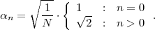 | (7.68) |
The inverse transform is given by
![N∑- 1 ( π ( 1))
s[n] = u[k ]⋅αk ⋅ cos -- k n+ -- .
k=0 N 2](VBpart1756x.png) | (7.69) |
The DCT-II is the most commonly used transform in image and video coding application. It is included in the following coding standards: JPEG [38], H.261 [35], H.262/MPEG-2 [39], H.263 [36], and MPEG-4 [31]. Although, the most recent video coding standard H.264/AVC [36] does not include a DCT as discussed above, it includes an integer approximation of the DCT that has similar properties, but can be implemented more efficiently and does not cause an accumulation of rounding errors inside the motion-compensation loop. The justification for the wide usage of the DCT includes the following points:
In contrast to the KLT, the basis vectors of the DCT are independent of the input source and there exist fast algorithms for computing the forward and inverse transforms. For zero-mean Gauss-Markov sources with large correlation coefficients ρ, the DCT-II basis vectors are a good approximation of the eigenvectors of the autocorrelation matrix RSS. If we neglect possible multiplications with -1, the basis vectors of the KLT for zero-mean Gauss-Markov sources approach the DCT-II basis vectors as the correlation coefficient ρ approaches one [2]. This is illustrated in Fig. 7.9. On the left side of this figure, the basis vectors of a KLT for zero-mean Gauss-Markov sources with a correlation coefficient of ρ = 0.9 are compared with the basis vectors of the DCT-II. On the right side of Fig. 7.9, the mean square difference δ(ρ) between the transform matrix of the DCT-II ADCT and the KLT transform matrix AKLT is shown as function of the correlation coefficient ρ. For this experiment, we used the KLT transform matrices AKLT for which the basis vectors (rows) are ordered in decreasing order of the associated eigenvalues and all entries in the first column are non-negative.
Fig. 7.9 Comparison of the basis vectors of the DCT-II and the KLT for zero-mean Gauss-Markov sources for a transform size N = 8: (left) basis vectors of the DCT-II and a KLT for ρ = 0.9; (right) mean square difference between the DCT-II and the KLT transform matrix as function of the correlation coefficient ρ.
As a simple transform coding example, we consider the Hadamard transform of the size N = 2 for a zero-mean Gauss-Markov process with a variance σS2 and a correlation coefficient ρ. The input vectors s and the orthogonal analysis transform matrix A are given by
![[ ] [ ]
s0 1-- 1 1
s = s1 and A = √2- 1 - 1 .](VBpart1777x.png) | (7.70) |
The analysis transform
![[ u ] 1 [ 1 1 ][ s ]
u = 0 = As = √-- 0
u1 2 1 - 1 s1](VBpart1778x.png) | (7.71) |
yields the transform coefficients
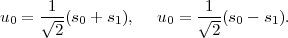 | (7.72) |
For the Hadamard transform, the synthesis transform matrix B is equal to the analysis transform matrix, B = AT = A.
The transform coefficient variances are given by
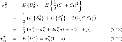
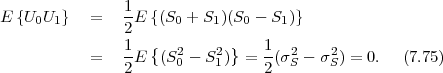
In the following, we consider entropy-constrained scalar quantization of the transform coefficients at high rates. The high-rate approximation of the operational distortion rate function for entropy-constrained scalar quantization of Gaussian sources is given by Di(Ri) = ε2σi22-2Ri with ε2 = πe∕6. The optimal bit allocation rule for high rates (cp. sec. 7.3.2) yields the component rates
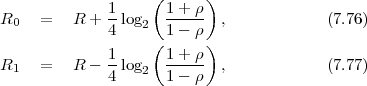
 log 2
log 2 bits larger than the rate R1 for the AC
coefficient u1. The high-rate operational distortion rate function for the
considered transform coder is given by
bits larger than the rate R1 for the AC
coefficient u1. The high-rate operational distortion rate function for the
considered transform coder is given by
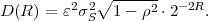 | (7.78) |
A comparison with the Shannon Lower bound (4.80) shows that, for high rates, the loss against the fundamental rate distortion bound is
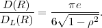 | (7.79) |
For zero-mean Gauss-Markov sources with ρ = 0.9 and high rates, the transform coding gain is about 3.61 dB, while the loss against the Shannon lower bound is about 5.14 dB. The transform coding gain can be increased by applying larger decorrelating transforms.
7.7 Summary of Transform Coding
In this chapter, we discussed transform coding with orthogonal block transforms. An orthogonal block transform of size N specifies a rotation or reflection of the coordinate system in the N-dimensional signal space. We showed that a transform coding system with an orthogonal block transform and scalar quantization of the transform coefficients represents a vector quantizer for which the quantization cells are hyperrectangles in the N-dimensional signal space. In contrast to scalar quantization in the original domain, the grid of quantization cells is not aligned with the coordinate axes of the original space. A decorrelation transform rotates the coordinate system toward the primary axes of the N-dimensional joint pdf, which has the effect that, for correlated sources, scalar quantization in the transform domain becomes more effective than in the original signal space.
The optimal distribution of the overall bit rate among the transform coefficients was discussed in some detail with the emphasis on Gaussian sources and high rates. In general, an optimal bit allocation is obtained if all component quantizers are operated at the same slope of their operational distortion rate functions. For high rates, this is equivalent to a bit allocation that yields equal component distortions. For stationary sources with memory the effect of the unitary transform is a nonuniform assignment of variances to the transform coefficients. This nonuniform distribution is the reason for the transform gain in case of optimal bit allocation.
The KLT was introduced as the transform that generates decorrelated transform coefficients. We have shown that the KLT is the optimal transform for Gaussian sources if we use the same type of optimal quantizers, with appropriately scaled reconstruction levels and decision thresholds, for all transform coefficients. For the example of Gaussian sources, we also derived the asymptotic operational distortion rate function for large transform sizes and high rates. It has been shown that, for zero-mean Gaussian sources and entropy-constrained scalar quantization, the distance of the asymptotic operational distortion rate function to the fundamental rate distortion bounds is basically reduced to the space-filling advantage of vector quantization.
In practical video coding systems, KLT’s are not used, since they are signal-dependent and cannot be implemented using fast algorithms. The most widely used transform is the DCT-II, which can be derived from the discrete Fourier transform (DFT) by introducing mirror symmetry with sample repetition at the signal boundaries and applying a DFT of double size. Due to the mirror symmetry, the DCT significantly reduces the blocking artifacts compared to the DFT. For zero-mean Gauss-Markov sources, the basis vectors of the KLT approach the basis vectors of the DCT-II as the correlation coefficient approaches one.
For highly-correlated sources, a transform coding system with a DCT-II and entropy-constrained scalar quantization of the transform coefficients is highly efficient in terms of both rate distortion performance and computational complexity.
This is the html version of the book:
Thomas Wiegand and Heiko Schwarz (2010): "Source Coding: Part I of Fundamentals of Source and Video Coding", Now Publishers, Foundations and Trends® in Signal Processing: Vol. 4: No 1-2, pp 1-222. (pdf version of the book)
8 Summary
The problem of communication may be posed as conveying source data with the highest fidelity possible without exceeding an available bit rate, or it may be posed as conveying the source data using the lowest bit rate possible while maintaining a specified reproduction fidelity. In either case, a fundamental trade-off is made between bit rate and signal fidelity. Source coding as described in this text provides the means to effectively control this trade-off.
Two types of source coding techniques are typically named: lossless and lossy coding. The goal of lossless coding is to reduce the average bit rate while incurring no loss in fidelity. Lossless coding can provide a reduction in bit rate compared to the original data, when the original signal contains dependencies or statistical properties that can be exploited for data compaction. The lower bound for the achievable bit rate of a lossless code is the discrete entropy rate of the source. Techniques that attempt to approach the entropy limit are called entropy coding algorithms. The presented entropy coding algorithms include Huffman codes, arithmetic codes, and the novel PIPE codes. Their application to discrete sources with and without consideration of statistical dependencies inside a source is described.
The main goal of lossy coding is to achieve lower bit rates than with lossless coding techniques while accepting some loss in signal fidelity. Lossy coding is the primary coding type for the compression of speech, audio, picture, and video signals, where an exact reconstruction of the source data is often not required. The fundamental limit for lossy coding algorithms is given by the rate distortion function, which specifies the minimum bit rate that is required for representing a source without exceeding a given distortion. The rate distortion function is derived as a mathematical function of the input source, without making any assumptions about the coding technique.
The process of incurring a reduction of signal fidelity is called quantization. Quantizers allow to effectively trade-off bit rate and signal fidelity and are at the core of every lossy source coding system. They can be classified into scalar and vector quantizers. For data containing none or little statistical dependencies, the combination of scalar quantization and scalar entropy coding is capable of providing a high coding efficiency at a low complexity level.
When the input data contain relevant statistical dependencies, these can be exploited via various techniques that are applied prior to or after scalar quantization. Prior to scalar quantization and scalar entropy coding, the statistical dependencies contained in the signal can be exploited through prediction or transforms. Since the scalar quantizer performance only depends on the marginal probability distribution of the input samples, both techniques, prediction and transforms, modify the marginal probability distribution of the samples to be quantized, in comparison to the marginal probability distribution of the input samples, via applying signal processing to two or more samples.
After scalar quantization, the applied entropy coding method could also exploit the statistical dependencies between the quantized samples. When the high rate assumptions are valid, it has been shown that this approach achieves a similar level of efficiency as techniques applied prior to scalar quantization. Such advanced entropy coding techniques are, however, associated with a significant complexity and, from practical experience, they appear to be inferior in particular at low bit rates.
The alternative to scalar quantization is vector quantization. Vector quantization allows the exploitation of statistical dependencies within the data without the application of any signal processing algorithms in advance of the quantization process. Moreover, vector quantization offers a benefit that is unique to this techniques as it is a property of the quantization in high-dimensional spaces: the space filling advantage. The space filling advantage is caused by the fact that a partitioning of high-dimensional spaces into hyperrectangles, as achieved by scalar quantization, does not represent the densest packing. However, this gain can be only achieved by significantly increasing the complexity in relation to scalar quantization. In practical coding systems, the space filling advantage is usually ignored. Vector quantization is typically only used with certain structural constraints, which significantly reduce the associated complexity.
The present text describes the subject of source coding for 1-d discrete-time signals. For the quantitative analysis of the efficiency of the presented coding techniques, the source signals are considered as realizations of simple stationary random processes. The second part of the monograph discusses the subject of video coding. There are several important differences between source coding of 1-d stationary model sources and the compression of natural camera-view video signals. The first and most obvious difference is that we move from 1-d to 2-d signals in case of picture coding and to 3-d signals in case of video coding. Hence, the 1-d concepts need to be extended accordingly. Another important difference is that the statistical properties of natural camera-view video signals are nonstationary and, at least to a significant extend, unknown in advance. For an efficient coding of video signals, the source coding algorithms need to be adapted to the local statistics of the video signal as we will discuss in the second part of this monograph.
This is the html version of the book:
Thomas Wiegand and Heiko Schwarz (2010): "Source Coding: Part I of Fundamentals of Source and Video Coding", Now Publishers, Foundations and Trends® in Signal Processing: Vol. 4: No 1-2, pp 1-222. (pdf version of the book)
References
[1] N. M. Abramson. Information Theory and Coding. McGraw-Hill, New York,
NY, USA, 1963.
[2] N. Ahmed, T. Natarajan, and K. R. Rao. Discrete Cosine Transform. IEEE
Transactions on Computers, 23(1):90–93, 1974.
[3] S. Arimoto. An Algorithm for Calculating the Capacity of an Arbitrary
Discrete Memoryless Channel. IEEE Transactions on Information Theory,
18:14–20, Jan. 1972.
[4] T. Berger. Rate Distortion Theory. Prentice-Hall, Englewood Cliffs, NJ, USA,
1971.
[5] J. Binia, M. Zakai, and J. Ziv. On the ϵ-Entropy and the Rate-Distortion
Function of Certain Non-Gaussian Processes. IEEE Transactions on
Information Theory, 20:514–524, July 1974.
[6] R. E. Blahut. Computation of Channel Capacity and Rate-Distortion
Functions. IEEE Transactions on Information Theory, 18:460–473, Apr. 1972.
[7] M. Burrows and D. Wheeler. A Block-Sorting Lossless Data Compression
Algorithm. Research Report 124, Digital Equipment Corporation, Palo Alto,
CA, USA, May 1994.
[8] P.-C. Chang and R. M. Gray. Gradient Algorithms for Designing Predictive
Vector Quantizers. IEEE Transactions on Acoustics, Speech and Signal
Processing, 34(4):679–690, Aug. 1986.
[9] P. A. Chou, T. Lookabaugh, and R. M. Gray. Entropy-Constrained Vector
Quantization. IEEE Transactions on Acoustics, Speech and Signal Processing,
37(1):31–42, Jan. 1989.
[10] R. J. Clarke. Transform Coding of Images. Academic Press, Orlando, Fla.,
1985.
[11] T. M. Cover and J. A. Thomas. Elements of Information Theory. John Wiley
and Sons, Hoboken, NJ, USA, 2006. 2nd edition.
[12] R. D. Dony and S. Haykin. Optimally Adaptive Transform Coding. IEEE
Transactions on Image Processing, 4(10):1358–1370, Oct. 1995.
[13] M. Effros, H. Feng, and K. Zeger. Suboptimality of the Karhunen-Loève
Transform for Transform Coding. IEEE Transactions on Information Theory,
50(8):1605–1619, Aug. 2004.
[14] R. G. Gallager. Information Theory and Reliable Communication. John Wiley
& Sons, New York, USA, 1968.
[15] R. G. Gallager. Variations on a Theme by Huffman. IEEE Transactions on
Information Theory, 24(6):668–674, Nov. 1978.
[16] A. Gersho and R. M. Gray. Vector Quantization and Signal Compression.
Kluwer Academic Publishers, Boston, Dordrecht, London, 1992.
[17] H. Gish and J. N. Pierce. Asymptotically Efficient Quantizing. IEEE
Transactions on Information Theory, 14:676–683, Sept. 1968.
[18] G. H. Golub and H. A. van der Vorst. Eigenvalue Computation in the 20th
Century. Journal of Computational and Applied Mathematics, 123:35–65, 2000.
[19] V. K. Goyal. High-Rate Transform Coding: How High is High, and Does it
Matter? In Proceedings of the IEEE International Symposium on Information
Theory, Sorento, Italy, June 2000.
[20] V. K. Goyal. Theoretical Foundations of Transform Coding. IEEE Signal
Processing Magazine, 18(5):9–21, Sept. 2001.
[21] V. K. Goyal, J. Zhuang, and M. Vetterli. Transform Coding with
Backward Adaptive Updates. IEEE Transactions on Information Theory,
46(4):1623–1633, July 2000.
[22] R. M. Gray. Source Coding Theory. Kluwer Academic Publishers, Norwell,
MA, USA, 1990.
[23] R. M. Gray. Toeplitz and Circulant Matrices: A Review. Foundations and
Trends in Communication and Information Theory, 2(3):155–329, 2005.
[24] R. M. Gray. Linear Predictive Coding and the Internet Protocol. Now
Publishers Inc, Boston-Delft, 2010.
[25] R. M. Gray and L. D. Davisson. Random Processes: A Mathematical Approach
for Engineers. Prentice Hall, Englewood Cliffs, NJ, USA, 1985.
[26] R. M. Gray and L. D. Davisson. An Introduction to Statistical Signal
Processing. Cambridge University Press, 2004.
[27] R. M. Gray and A. H. Gray. Asymptotically Optimal Quantizers. IEEE
Transactions on Information Theory, 23:143–144, Jan. 1977.
[28] R. M. Gray and D. L. Neuhoff. Quantization. IEEE Transactions on
Information Theory, 44(6):2325–2383, Oct. 1998.
[29] U. Grenander and G. Szegö. Toeplitz Forms and Their Applications.
University of California Press, Berkeley and Los Angeles, USA, 1958.
[30] D. A. Huffman. A Method for the Construction of Minimum Redundancy
Codes. Proc. IRE, pages 1098–1101, Sept. 1952.
[31] ISO/IEC. Coding of Audio-Visual Objects — Part 2: Visual. ISO/IEC 14496-2,
Apr. 1999.
[32] ITU-T. Narrow-Band Visual Telephone Systems and Terminal Equipment.
ITU-T Rec. H.320, 1999.
[33] ITU-T. Packet-Based Multimedia Communications Systems. ITU-T Rec.
H.323, 1998.
[34] ITU-T. Terminal for Low Bit Rate Multimedia Communication. ITU-T Rec.
H.324, 1996.
[35] ITU-T. Video Codec for Audiovisual Services at p × 64 kbit/s. ITU-T Rec.
H.261, Mar. 1993.
[36] ITU-T and ISO/IEC. Advanced Video Coding for Generic Audiovisual
Services. ITU-T Rec. H.264 and ISO/IEC 14496-10 (MPEG-4 AVC), Mar.
2010.
[37] ITU-T and ISO/IEC. Generic Coding of Moving Pictures and Asociated Audio
Information — Part 1: Systems. ITU-T Rec. H.222.0 and ISO/IEC 13818-1
(MPEG-2 Systems), Nov. 1994.
[38] ITU-T and ISO/IEC. Digital Compression and Coding of Continuous-Tone
Still Images. ITU-T Rec. T.81 and ISO/IEC 10918-1 (JPEG), Sept. 1992.
[39] ITU-T and ISO/IEC. Generic Coding of Moving Pictures and Associated Audio
Information — Part 2: Video. ITU-T Rec. H.262 and ISO/IEC 13818-2, Nov.
1994.
[40] ITU-T and ISO/IEC. Lossless and Near-Lossless Compression of
Continuous-Tone Still Images. ITU-T Rec. T.87 and ISO/IEC 14495-1
(JPEG-LS), June 1998.
[41] ITU-T and ISO/IEC. JPEG 2000 Image Coding System – Core Coding System.
ITU-T Rec. T.800 and ISO/IEC 15444-1 (JPEG 2000), 2002.
[42] ITU-T and ISO/IEC. JPEG XR Image Coding System – Image Coding
Specification. ITU-T Rec. T.832 and ISO/IEC 29199-2 (JPEG XR), 2009.
[43] C. G. J. Jacobi. Über ein leichtes Verfahren, die in der Theorie der
Säcularströmungen vorkommenden Gleichungen numerisch aufzulösen. Journal
für reine und angewandte Mathematik, 30:51–94, 1846.
[44] N. S. Jayant and P. Noll. Digital Coding of Waveforms. Prentice-Hall,
Englewood Cliffs, NJ, USA, 1994.
[45] A. N. Kolmogorov. Grundbegriffe der Wahrscheinlichkeitsrechnung. Springer,
Berlin, Germany, 1933. An English translation by N. Morrison appeared under
the title Foundations of the Theory of Probability (Chelsea, New York) in 1950,
with a second edition in 1956.
[46] Y. Linde, A. Buzo, and R. M. Gray. An Algorithm for Vector Quantizer
Design. IEEE Transactions on Communications, 28(1):84–95, Jan. 1980.
[47] T. Linder and R. Zamir. On the Asymptotic Tightness of the Shannon Lower
Bound. IEEE Transactions on Information Theory, 40(6):2026–2031, Nov.
1994.
[48] Y. N. Linkov. Evaluation of Epsilon Entropy of Random Variables for Small
Esilon. Problems of Information Transmission, 1:12–18, 1965.
[49] S. P. Lloyd. Least Squares Quantization in PCM. IEEE Transactions on
Information Theory, 28:127–135, Mar. 1982. Unpublished Bell Laboratories
Technical Note, 1957.
[50] T. D. Lookabaugh and R. M. Gray. High-Resolution Quantization Theory and
the Vector Quantizer Advantage. IEEE Transactions on Information Theory,
35(5):1020–1033, Sept. 1989.
[51] J. Makhoul. Linear Prediction: A Tutorial Review. Proceedings of the IEEE,
63(4):561–580, Apr. 1975.
[52] J. Makhoul, S. Roucos, and H. Gish. Vector Quantization in Speech Coding.
Proceedings of the IEEE, 73(11):1551–1587, Nov. 1985.
[53] H. S. Malvar. Signal Processing with Lapped Transforms. Artech House,
Norwood, MA, USA, 1992.
[54] D. Marpe, H. Schwarz, and T. Wiegand. Probability Interval Partitioning
Entropy Codes. Submitted to IEEE Transactions on Information Theory, 2010.
Available at http://iphome.hhi.de/marpe/download/pipe-subm-ieee10.pdf.
[55] D. Marpe, H. Schwarz, and T. Wiegand. Context-Adaptive Binary
Arithmetic Coding for H.264/AVC. IEEE Transactions on Circuits and
Systems for Video Technology, 13(7):620–636, July 2003.
[56] J. Max. Quantizing for Minimum Distortion. IRE Transactions on Information
Theory, 6(1):7–12, Mar. 1960.
[57] R. A. McDonald and P. M. Schultheiss. Information Rates of Gaussian Signals
under Criteria Constraining the Error Spectrum. Proceedings of the IEEE,
52:415–416, 1964.
[58] A. Moffat, R. M. Neil, and I. H. Witten. Arithmetic Coding Revisited. ACM
Transactions on Information Systems, 16(3):256–294, July 1998.
[59] P. F. Panter and W. Dite. Quantization Distortion in Pulse Code Modulation
with Nonuniform Spacing of Levels. Proc. IRE, 39:44–48, Jan. 1951.
[60] A. Papoulis and S. U. Pillai. Probability, Random Variables and Stochastic
Processes. McGraw-Hill, New York, NY, USA, 2002.
[61] R. Pasco. Source Coding Algorithms for Fast Data Compression. Ph.D.
dissertation, Stanford University, 1976.
[62] R. L. D. Queiroz and T. D. Tran. Lapped Transforms for Image Compression.
In The Transform and Data Compression Handbook, pages 197–265, Boca
Raton, FL, 2001. CRC.
[63] J. Rissanen. Generalized Kraft Inequality and Arithmetic Coding. IBM J.
Res. Develop., 20:198–203, 1976.
[64] J. Rosenberg, H. Schulzrinne, G. Camarillo, A. Johnston, J. Peterson,
R. Sparks, M. Handley, and E. Schooler. SIP: Session Initiation Protocol.
IETF RFC 3261, 2002.
[65] A. Said. Arithmetic Coding. In K. Sayood, editor, Lossless Compression
Handbook. Academic Press, San Diego, CA, 2003.
[66] S. A. Savari and R. G. Gallager. Generalized Tunstall Codes for Soures with
Memory. IEEE Transactions on Information Theory, 43(2):658–668, Mar. 1997.
[67] K. Sayood, editor. Lossless Compression Handbook. Academic Press, San
Diego, CA, 2003.
[68] H. Schulzrinne, S. Casner, R. Frederick, and V. Jacobson. RTP: A Transport
Protocol for Real-Time Applications. IETF RFC 1889, 1996.
[69] C. E. Shannon. A Mathematical Theory of Communication. The Bell System
Technical Journal, 27(3):2163–2177, July 1948.
[70] C. E. Shannon. Coding Theorems for a Discrete Source with a Fidelity
Criterion. IRE National Convention Record, Part 4, pages 142–163, 1959.
[71] Y. Shoham and A. Gersho. Efficient Bit Allocation for an Arbitrary Set of
Quantizers. IEEE Transactions on Acoustics, Speech and Signal Processing,
36:1445–1453, Sept. 1988.
[72] D. S. Taubman and M. M. Marcellin. JPEG2000: Image Compression
Fundamentals, Standards and Practice. Kluwer Academic Publishers, 2001.
[73] B. P. Tunstall. Synthesis of Noiseless Compression Codes. Ph.D. dissertation,
Georgia Inst. Technol., 1967.
[74] B. E. Usevitch. A Tutorial on Mondern Lossy Wavelet Image Compression:
Foundations of JPEG 2000. IEEE Signal Processing Magazine, 18(5):22–35,
Sept. 2001.
[75] P. P. Vaidyanathan. The Theory of Linear Prediction. Morgan & Claypool
Publishers, 2008.
[76] M. Vetterli. Wavelets, Approximation, and Compression. IEEE Signal
Processing Magazine, 18(5):59–73, Sept. 2001.
[77] M. Vetterli and J. Kovacevic. Wavelets and Subband Coding. Prentice-Hall,
Englewood Cliffs, NJ, 1995.
[78] I. H. Witten, R. M. Neal, and J. G. Cleary. Arithmetic Coding for Data
Compression. Communications of the ACM, 30(6):520–540, June 1987.
[79] J. Ziv and A. Lempel. A Universal Algorithm for Data Compression. IEEE
Transactions on Information Theory, 23(3):337–343, May 1977.